Page 184 - Applied statistics and probability for engineers

162 Chapter 5/Joint Probability Distributions

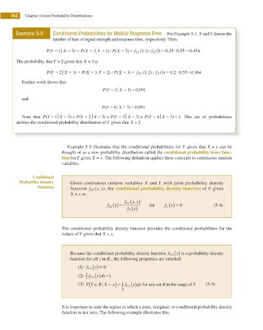
Example 5-5 Conditional Probabilities for Mobile Response Time For Example 5-1, X and Y denote the
number of bars of signal strength and response time, respectively. Then,

P Y 51u X 53 )5 P X 53 ,Y 51 ) / P X 53 )5 f XY (3 , ) / f X ( )5 0 25 0 55 5 0 4554
(
(
(
/
.
.
1
3
.
The probability that Y = 2 given that X = 3 is

P Y 5 2 u X 53 )5 P X 53 ,Y 5 2 ) / P X 53 )5 f XY (3 , ) / f X ( )5 0 2 0 55 50 3644
2
3
(
(
.
.
(
/
.
Further work shows that
P Y = 3u X = 3 ) = 0 .091
(
and
P Y = 4 u X = 3 ) = 0 .091.
(
Note that P Y = 1⏐ X = 3 ) + P Y = 2⏐ X = 3 ) + P Y = 3⏐ X = 3 ) + P Y = 4⏐ X = 3 ) = 1. This set of probabilities
(
(
(
(

deines the conditional probability distribution of Y given that X = 3.
Example 5-5 illustrates that the conditional probabilities for Y given that X = x can be
thought of as a new probability distribution called the conditional probability mass func-
tion for Y given X = x. The following deinition applies these concepts to continuous random

variables.
Conditional
Probability Density Given continuous random variables X and Y with joint probability density
Function function f XY ( x y), the conditional probability density function of Y given
,
X = x is
f XY ( x, y )
f Y x u ( y)5 f X ( x) for f X ( x). 0 (5-4)
The conditional probability density function provides the conditional probabilities for the
values of Y given that X = x.

Because the conditional probability density function f Y x|| ( y) is a probability density
function for all y in R x , the following properties are satisi ed:
(1) f Y x| ( )
y $ 0
(2) f Y x| ( )
∫
y dy51
(
(3) P Y ∈ B X 5 x)5 ∫ f Y x ( ) B in the range of Y (5-5)
u
y dy for any set
u
B
It is important to state the region in which a joint, marginal, or conditional probability density
function is not zero. The following example illustrates this.