Page 225 - Applied statistics and probability for engineers

Section 6-1/Numerical Summaries of Data 203

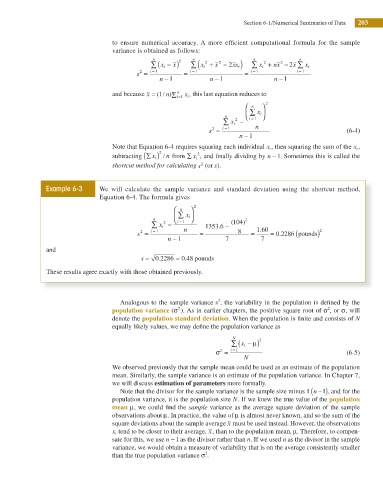
to ensure numerical accuracy. A more efi cient computational formula for the sample
variance is obtained as follows:
n n n n
∑ ( x i − ) 2 ∑ x i ( 2 + x − 2 xx i) ∑ x i + nx − 2 x ∑ x i
2
2
2
x
s = i = 1 = i = 1 = i = 1 i i = 1
2
−
−
n 1 n 1 n − 1
and because x = (1/ n) Σ i=1 x i , this last equation reduces to
n
⎛ n ⎞ 2
⎜ ∑ x i ⎟
n i ⎝ = 1 ⎠
∑ x i −
2
2
s = i = 1 n (6-4)
−
n 1
Note that Equation 6-4 requires squaring each individual x , i then squaring the sum of the x , i
2
) / n from ∑ x i , and i nally dividing by n − 1. Sometimes this is called the
2
subtracting ∑ ( x i
2
shortcut method for calculating s (or s).
Example 6-3 We will calculate the sample variance and standard deviation using the shortcut method,
Equation 6-4. The formula gives
⎛ n ⎞ 2
⎜ ∑ x i ⎟
n i ⎝ = 1 ⎠ 2
∑ x i − 1353 6 − ( 104)
2
.
.
0 22866 pounds)
s = i = 1 n = 8 = 1 60 = . ( 2
2
−
n 1 7 7
and
.
.
s = 0 2286 = 0 48 pounds
These results agree exactly with those obtained previously.
2
Analogous to the sample variance s , the variability in the population is dei ned by the
population variance (σ 2 ). As in earlier chapters, the positive square root of σ , or σ, will
2

denote the population standard deviation. When the population is inite and consists of N
equally likely values, we may deine the population variance as

N 2
∑ (x i − ) μ
σ = i = 1 (6-5)
2
N
We observed previously that the sample mean could be used as an estimate of the population
mean. Similarly, the sample variance is an estimate of the population variance. In Chapter 7,
we will discuss estimation of parameters more formally.
(
Note that the divisor for the sample variance is the sample size minus 1 n − ) 1 , and for the
population variance, it is the population size N. If we knew the true value of the population
mean μ, we could i nd the sample variance as the average square deviation of the sample
observations about μ. In practice, the value of μ is almost never known, and so the sum of the
square deviations about the sample average x must be used instead. However, the observations
x i tend to be closer to their average, x, than to the population mean, μ. Therefore, to compen-
sate for this, we use n − 1 as the divisor rather than n. If we used n as the divisor in the sample
variance, we would obtain a measure of variability that is on the average consistently smaller
2
than the true population variance σ .