Page 226 - Applied statistics and probability for engineers

204 Chapter 6/Descriptive Statistics

Another way to think about this is to consider the sample variance s 2 as being based
on n − 1 degrees of freedom. The term degrees of freedom results from the fact that the n
deviations x 1 − , − x,… , x n − x always sum to zero, and so specifying the values of any
x x 2
n −1 of these quantities automatically determines the remaining one. This was illustrated in
Table 6-1. Thus, only n −1 of the n deviations, x i − x, are freely determined. We may think
of the number of degrees of freedom as the number of independent pieces of information
in the data.
In addition to the sample variance and sample standard deviation, the sample range, or the
difference between the largest and smallest observations, is often a useful measure of vari-
ability. The sample range is deined as follows.

Sample Range
If the n observations in a sample are denoted by x , x , … , x , the sample range is
2
1
n
r = max x i ( ) − min x i ( ) (6-6)

For the pull-off force data, the sample range is r = 13 . −12 . = . . Generally, as the variability
3
3
1
6
in sample data increases, the sample range increases.
The sample range is easy to calculate, but it ignores all of the information in the sample
data between the largest and smallest values. For example, the two samples 1, 3, 5, 8, and 9
and 1, 5, 5, 5, and 9 both have the same range (r = 8 ). However, the standard deviation of the
irst sample is s 1 = 3 35 , while the standard deviation of the second sample is s 2 = 2 83. The
.
.
variability is actually less in the second sample.
Sometimes when the sample size is small, say n < 8 or 10 , the information loss associated
with the range is not too serious. For example, the range is used widely in statistical quality
control where sample sizes of 4 or 5 are fairly common. We will discuss some of these appli-
cations in Chapter 15.
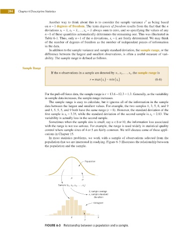
In most statistics problems, we work with a sample of observations selected from the
population that we are interested in studying. Figure 6-3 illustrates the relationship between
the population and the sample.

Population

m
s
, x , x , … , x )
Sample (x 1 2 3 n
x, sample average
s, sample standard
deviation
Histogram

x x
s
FIGURE 6-3 Relationship between a population and a sample.