Page 231 - Applied statistics and probability for engineers

Section 6-2/Stem-and-Leaf Diagrams 209

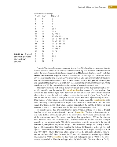
Stem-and-leaf of Strength
N = 80 Leaf Unit = 1.0
1 7 6
2 8 7
3 9 7
5 10 1 5
8 11 0 5 8
11 12 0 1 3
17 13 1 3 3 4 5 5
25 14 1 2 3 5 6 8 9 9
37 15 0 0 1 3 4 4 6 7 8 8 8 8
(10) 16 0 0 0 3 3 5 7 7 8 9
33 17 0 1 1 2 4 4 5 6 6 8
23 18 0 0 1 1 3 4 6
16 19 0 3 4 6 9 9
10 20 0 1 7 8
FIGURE 6-6 A typical 6 21 8
computer-generated 5 22 1 8 9
stem-and-leaf 2 23 7
diagram. 1 24 5

Figure 6-6 is a typical computer-generated stem-and-leaf display of the compressive strength
data in Table 6-2. The software uses the same stems as in Fig. 6-4. Note also that the computer
orders the leaves from smallest to largest on each stem. This form of the plot is usually called an
ordered stem-and-leaf diagram. This is not usually used when the plot is constructed manu-
ally because it can be time-consuming. The computer also adds a column to the left of the stems
that provides a count of the observations at and above each stem in the upper half of the display
and a count of the observations at and below each stem in the lower half of the display. At the
middle stem of 16, the column indicates the number of observations at this stem.
The ordered stem-and-leaf display makes it relatively easy to ind data features such as per-
centiles, quartiles, and the median. The sample median is a measure of central tendency that
divides the data into two equal parts, half below the median and half above. If the number of
observations is even, the median is halfway between the two central values. From Fig. 6-6 we
)
(
/
=
.
+
ind the 40th and 41st values of strength as 160 and 163, so the median is 160 163 2 161 5.
If the number of observations is odd, the median is the central value. The sample mode is the
most frequently occurring data value. Figure 6-6 indicates that the mode is 158; this value
occurs four times, and no other value occurs as frequently in the sample. If there were more
than one value that occurred four times, the data would have multiple modes.
We can also divide data into more than two parts. When an ordered set of data is divided
into four equal parts, the division points are called quartiles. The irst or lower quartile, q 1 ,
is a value that has approximately 25% of the observations below it and approximately 75%
of the observations above. The second quartile, q 2 , has approximately 50% of the observa-
tions below its value. The second quartile is exactly equal to the median. The third or upper
quartile, q 3 , has approximately 75% of the observations below its value. As in the case of
the median, the quartiles may not be unique. The compressive strength data in Fig. 6-6 con-
(
/
tain n = 80 observations. Therefore, calculate the irst and third quartiles as the n + ) 1 4 and
(
.
1 4 ordered observations and interpolate as needed, for example, 80 1 4+ ) /
3 n + ) / ( = 20 25
(
+ )
.
and 3 80 1 4 = 60 75. Therefore, interpolating between the 20th and 21st ordered observa-
/
tion we obtain q 1 = 143 50. and between the 60th and 61st observation we obtain q 3 = 181 00. .
In general, the 100kth percentile is a data value such that approximately 100k% of the obser-
(
vations are at or below this value and approximately 100 1− ) k % of them are above it. Finally,