Page 234 - Applied statistics and probability for engineers

212 Chapter 6/Descriptive Statistics

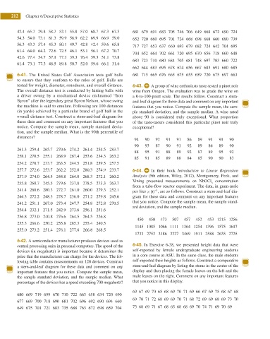
42.4 65.7 29.8 58.7 52.1 55.8 57.0 68.7 67.3 67.3 681 679 691 683 705 746 706 649 668 672 690 724
54.3 54.0 73.1 81.3 59.9 56.9 62.2 69.9 66.9 59.0 652 720 660 695 701 724 668 698 668 660 680 739
56.3 43.3 57.4 45.3 80.1 49.7 42.8 42.4 59.6 65.8 717 727 653 637 660 693 679 682 724 642 704 695
61.4 64.0 64.2 72.6 72.5 46.1 53.1 56.1 67.2 70.7
704 652 664 702 661 720 695 670 656 718 660 648
42.6 77.4 54.7 57.1 77.3 39.3 76.4 59.3 51.1 73.8
683 723 710 680 684 705 681 748 697 703 660 722
61.4 73.1 77.3 48.5 89.8 50.7 52.0 59.6 66.1 31.6
662 644 683 695 678 674 656 667 683 691 680 685
6-41. The United States Golf Association tests golf balls 681 715 665 676 665 675 655 659 720 675 697 663
to ensure that they conform to the rules of golf. Balls are
tested for weight, diameter, roundness, and overall distance. 6-43. A group of wine enthusiasts taste-tested a pinot noir
The overall distance test is conducted by hitting balls with wine from Oregon. The evaluation was to grade the wine on
a driver swung by a mechanical device nicknamed “Iron a 0-to-100-point scale. The results follow. Construct a stem-
Byron” after the legendary great Byron Nelson, whose swing and-leaf diagram for these data and comment on any important
the machine is said to emulate. Following are 100 distances features that you notice. Compute the sample mean, the sam-
(in yards) achieved by a particular brand of golf ball in the ple standard deviation, and the sample median. A wine rated
overall distance test. Construct a stem-and-leaf diagram for above 90 is considered truly exceptional. What proportion
these data and comment on any important features that you of the taste-tasters considered this particular pinot noir truly
notice. Compute the sample mean, sample standard devia- exceptional?
tion, and the sample median. What is the 90th percentile of
distances?
94 90 92 91 91 86 89 91 91 90
90 93 87 90 91 92 89 86 89 90
261.3 259.4 265.7 270.6 274.2 261.4 254.5 283.7
88 95 91 88 89 92 87 89 95 92
258.1 270.5 255.1 268.9 267.4 253.6 234.3 263.2
85 91 85 89 88 84 85 90 90 83
254.2 270.7 233.7 263.5 244.5 251.8 259.5 257.5
257.7 272.6 253.7 262.2 252.0 280.3 274.9 233.7 6-44. In their book Introduction to Linear Regression
237.9 274.0 264.5 244.8 264.0 268.3 272.1 260.2 Analysis (5th edition, Wiley, 2012), Montgomery, Peck, and
Vining presented measurements on NbOCl concentration
255.8 260.7 245.5 279.6 237.8 278.5 273.3 263.7 3
from a tube-low reactor experiment. The data, in gram-mole
241.4 260.6 280.3 272.7 261.0 260.0 279.3 252.1 per liter × 10 , are as follows. Construct a stem-and-leaf dia-
−3
244.3 272.2 248.3 278.7 236.0 271.2 279.8 245.6 gram for these data and comment on any important features
241.2 251.1 267.0 273.4 247.7 254.8 272.8 270.5 that you notice. Compute the sample mean, the sample stand-
ard deviation, and the sample median.
254.4 232.1 271.5 242.9 273.6 256.1 251.6
256.8 273.0 240.8 276.6 264.5 264.5 226.8
450 450 473 507 457 452 453 1215 1256
255.3 266.6 250.2 255.8 285.3 255.4 240.5
1145 1085 1066 1111 1364 1254 1396 1575 1617
255.0 273.2 251.4 276.1 277.8 266.8 268.5
1733 2753 3186 3227 3469 1911 2588 2635 2725
6-42. A semiconductor manufacturer produces devices used as
central processing units in personal computers. The speed of the 6-45. In Exercise 6-38, we presented height data that were
devices (in megahertz) is important because it determines the self-reported by female undergraduate engineering students
price that the manufacturer can charge for the devices. The fol- in a core course at ASU. In the same class, the male students
lowing table contains measurements on 120 devices. Construct self-reported their heights as follows. Construct a comparative
a stem-and-leaf diagram for these data and comment on any stem-and-leaf diagram by listing the stems in the center of the
important features that you notice. Compute the sample mean, display and then placing the female leaves on the left and the
the sample standard deviation, and the sample median. What male leaves on the right. Comment on any important features
percentage of the devices has a speed exceeding 700 megahertz? that you notice in this display.

69 67 69 70 65 68 69 70 71 69 66 67 69 75 68 67 68
680 669 719 699 670 710 722 663 658 634 720 690
69 70 71 72 68 69 69 70 71 68 72 69 69 68 69 73 70
677 669 700 718 690 681 702 696 692 690 694 660
649 675 701 721 683 735 688 763 672 698 659 704 73 68 69 71 67 68 65 68 68 69 70 74 71 69 70 69