Page 232 - Applied statistics and probability for engineers

210 Chapter 6/Descriptive Statistics

1
we may use the interquartile range, dei ned as IQR = q 3 − q , as a measure of variability. The
interquartile range is less sensitive to the extreme values in the sample than is the ordinary
sample range.
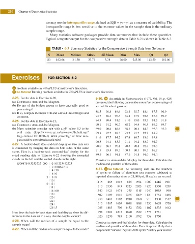
Many statistics software packages provide data summaries that include these quantities.
Typical computer output for the compressive strength data in Table 6-2 is shown in Table 6-3.

5"#-& t 6-3 Summary Statistics for the Compressive Strength Data from Software

N Mean Median StDev SE Mean Min Max Q1 Q3
80 162.66 161.50 33.77 3.78 76.00 245.00 143.50 181.00

Exercises FOR SECTION 6-2

Problem available in WileyPLUS at instructor’s discretion.
Tutoring problem available in WileyPLUS at instructor’s discretion.
6-25. For the data in Exercise 6-20, 6-30. An article in Technometrics (1977, Vol. 19, p. 425)
(a) Construct a stem-and-leaf diagram. presented the following data on the motor fuel octane ratings of
(b) Do any of the bridges appear to have unusually good or several blends of gasoline:
poor ratings?
88.5 98.8 89.6 92.2 92.7 88.4 87.5 90.9
(c) If so, compute the mean with and without these bridges and
comment. 94.7 88.3 90.4 83.4 87.9 92.6 87.8 89.9
6-26. For the data in Exercise 6-21, 84.3 90.4 91.6 91.0 93.0 93.7 88.3 91.8
(a) Construct a stem-and-leaf diagram. 90.1 91.2 90.7 88.2 94.4 96.5 89.2 89.7
(b) Many scientists consider rain with a pH below 5.3 to be 89.0 90.6 88.6 88.5 90.4 84.3 92.3 92.2
acid rain (http://www.ec.gc.ca/eau-water/default.asp? 89.8 92.2 88.3 93.3 91.2 93.2 88.9
lang=En&n=FDF30C16-1). What percentage of these sam-
91.6 87.7 94.2 87.4 86.7 88.6 89.8
ples could be considered as acid rain?
90.3 91.1 85.3 91.1 94.2 88.7 92.7
6-27. A back-to-back stem-and-leaf display on two data sets
90.0 86.7 90.1 90.5 90.8 92.7 93.3
is conducted by hanging the data on both sides of the same
91.5 93.4 89.3 100.3 90.1 89.3 86.7
stems. Here is a back-to-back stem-and-leaf display for the
cloud seeding data in Exercise 6-22 showing the unseeded 89.9 96.1 91.1 87.6 91.8 91.0 91.0
clouds on the left and the seeded clouds on the right. Construct a stem-and-leaf display for these data. Calculate the
65098754433332221000 | 0 | 01233492223 median and quartiles of these data.
| 2 | 00467703
| 4 | 39 6-31. The following data are the numbers
| 6 | 0 of cycles to failure of aluminum test coupons subjected to
3 | 8 | 8 repeated alternating stress at 21,000 psi, 18 cycles per second.
| 10 | 1115 865 1015 885 1594 1000 1416 1501
0 | 12 |
| 14 | 1310 2130 845 1223 2023 1820 1560 1238
| 16 | 60 1540 1421 1674 375 1315 1940 1055 990
| 18 | 1502 1109 1016 2265 1269 1120 1764 1468
| 20 | 1258 1481 1102 1910 1260 910 1330 1512
| 22 |
| 24 | 1315 1567 1605 1018 1888 1730 1608 1750
| 26 | 5 1085 1883 706 1452 1782 1102 1535 1642
How does the back-to-back stem-and-leaf display show the dif- 798 1203 2215 1890 1522 1578 1781
ferences in the data set in a way that the dotplot cannot? 1020 1270 785 2100 1792 758 1750
6-28. When will the median of a sample be equal to the
Construct a stem-and-leaf display for these data. Calculate the
sample mean?
median and quartiles of these data. Does it appear likely that a
6-29. When will the median of a sample be equal to the mode? coupon will “survive” beyond 2000 cycles? Justify your answer.