Page 235 - Applied statistics and probability for engineers

Section 6-3/Frequency Distributions and Histograms 213

6-3 Frequency Distributions and Histograms

A frequency distribution is a more compact summary of data than a stem-and-leaf diagram. To
construct a frequency distribution, we must divide the range of the data into intervals, which are
usually called class intervals, cells, or bins. If possible, the bins should be of equal width in order
to enhance the visual information in the frequency distribution. Some judgment must be used in
selecting the number of bins so that a reasonable display can be developed. The number of bins
depends on the number of observations and the amount of scatter or dispersion in the data. A fre-
quency distribution that uses either too few or too many bins will not be informative. We usually

ind that between 5 and 20 bins is satisfactory in most cases and that the number of bins should
increase with n. Several sets of rules can be used to determine the member of bins in a histogram.
However, choosing the number of bins approximately equal to the square root of the number of
observations often works well in practice.
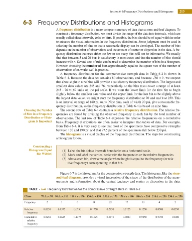
A frequency distribution for the comprehensive strength data in Table 6-2 is shown in
Table 6-4. Because the data set contains 80 observations, and because 80 ≃ 9, we suspect
that about eight to nine bins will provide a satisfactory frequency distribution. The largest and
smallest data values are 245 and 76, respectively, so the bins must cover a range of at least
=
245 − 76 169 units on the psi scale. If we want the lower limit for the i rst bin to begin
slightly below the smallest data value and the upper limit for the last bin to be slightly above
the largest data value, we might start the frequency distribution at 70 and end it at 250. This
is an interval or range of 180 psi units. Nine bins, each of width 20 psi, give a reasonable fre-
quency distribution, so the frequency distribution in Table 6-4 is based on nine bins.
Choosing the Number The second row of Table 6-4 contains a relative frequency distribution. The relative fre-
of Bins in a Frequency quencies are found by dividing the observed frequency in each bin by the total number of
Distribution or Histo- observations. The last row of Table 6-4 expresses the relative frequencies on a cumulative
gram is Important basis. Frequency distributions are often easier to interpret than tables of data. For example,
from Table 6-4, it is very easy to see that most of the specimens have compressive strengths
between 130 and 190 psi and that 97.5 percent of the specimens fall below 230 psi.
The histogram is a visual display of the frequency distribution. The steps for constructing
a histogram follow.

Constructing a
Histogram (Equal (1) Label the bin (class interval) boundaries on a horizontal scale.
Bin Widths) (2) Mark and label the vertical scale with the frequencies or the relative frequencies.
(3) Above each bin, draw a rectangle where height is equal to the frequency (or rela-
tive frequency) corresponding to that bin.

Figure 6-7 is the histogram for the compression strength data. The histogram, like the stem-
and-leaf diagram, provides a visual impression of the shape of the distribution of the meas-
urements and information about the central tendency and scatter or dispersion in the data.

5 6-4 Frequency Distribution for the Compressive Strength Data in Table 6-2
Class 70 Ä < 90 90 Ä <x 110 110 Ä <x 130 130 Ä <x 150 150 Ä < 170 170 Ä < 190 190 Ä < 210 210 Ä < 230 230 Ä < 250
x
x
x
x
x
x
Frequency 2 3 6 14 22 17 10 4 2
Relative 0.0250 0.0375 0.0750 0.1750 0.2750 0.2125 0.1250 0.0500 0.0250
frequency
Cumulative 0.0250 0.0625 0.1375 0.3125 0.5875 0.8000 0.9250 0.9750 1.0000
relative
frequency