Page 240 - Applied statistics and probability for engineers

218 Chapter 6/Descriptive Statistics

120

110
250 * 245
237.25 237
1.5 IQR 100
200
181 q = 181 Quality index 90
3
Strength 143.5 IQR 150 q = 161.5
2
q = 143.5
1
80
1.5 IQR
100 97
87.25 * 87 70
* 76 1 2 3
Plant
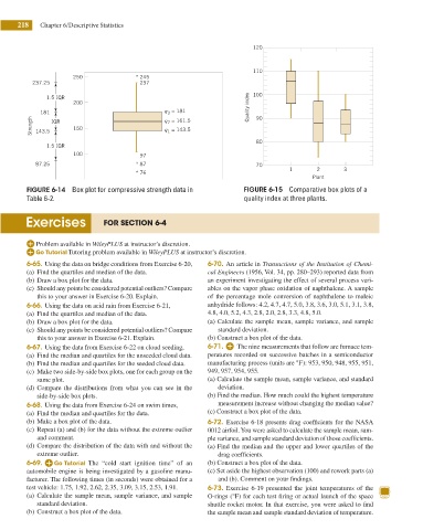
FIGURE 6-14 Box plot for compressive strength data in FIGURE 6-15 Comparative box plots of a
Table 6-2. quality index at three plants.

Exercises FOR SECTION 6-4

Problem available in WileyPLUS at instructor’s discretion.
Tutoring problem available in WileyPLUS at instructor’s discretion.
6-65. Using the data on bridge conditions from Exercise 6-20, 6-70. An article in Transactions of the Institution of Chemi-
(a) Find the quartiles and median of the data. cal Engineers (1956, Vol. 34, pp. 280–293) reported data from
(b) Draw a box plot for the data. an experiment investigating the effect of several process vari-
(c) Should any points be considered potential outliers? Compare ables on the vapor phase oxidation of naphthalene. A sample
this to your answer in Exercise 6-20. Explain. of the percentage mole conversion of naphthalene to maleic
6-66. Using the data on acid rain from Exercise 6-21, anhydride follows: 4.2, 4.7, 4.7, 5.0, 3.8, 3.6, 3.0, 5.1, 3.1, 3.8,
(a) Find the quartiles and median of the data. 4.8, 4.0, 5.2, 4.3, 2.8, 2.0, 2.8, 3.3, 4.8, 5.0.
(b) Draw a box plot for the data. (a) Calculate the sample mean, sample variance, and sample
(c) Should any points be considered potential outliers? Compare standard deviation.
this to your answer in Exercise 6-21. Explain. (b) Construct a box plot of the data.
6-67. Using the data from Exercise 6-22 on cloud seeding, 6-71. The nine measurements that follow are furnace tem-
(a) Find the median and quartiles for the unseeded cloud data. peratures recorded on successive batches in a semiconductor
(b) Find the median and quartiles for the seeded cloud data. manufacturing process (units are °F): 953, 950, 948, 955, 951,
(c) Make two side-by-side box plots, one for each group on the 949, 957, 954, 955.
same plot. (a) Calculate the sample mean, sample variance, and standard
(d) Compare the distributions from what you can see in the deviation.
side-by-side box plots. (b) Find the median. How much could the highest temperature
6-68. Using the data from Exercise 6-24 on swim times, measurement increase without changing the median value?
(a) Find the median and quartiles for the data. (c) Construct a box plot of the data.
(b) Make a box plot of the data. 6-72. Exercise 6-18 presents drag coeficients for the NASA
(c) Repeat (a) and (b) for the data without the extreme outlier 0012 airfoil. You were asked to calculate the sample mean, sam-
and comment. ple variance, and sample standard deviation of those coeficients.
(d) Compare the distribution of the data with and without the (a) Find the median and the upper and lower quartiles of the
extreme outlier. drag coeficients.
6-69. The “cold start ignition time” of an (b) Construct a box plot of the data.
automobile engine is being investigated by a gasoline manu- (c) Set aside the highest observation (100) and rework parts (a)
facturer. The following times (in seconds) were obtained for a and (b). Comment on your indings.
test vehicle: 1.75, 1.92, 2.62, 2.35, 3.09, 3.15, 2.53, 1.91. 6-73. Exercise 6-19 presented the joint temperatures of the
(a) Calculate the sample mean, sample variance, and sample O-rings (°F) for each test iring or actual launch of the space
standard deviation. shuttle rocket motor. In that exercise, you were asked to ind
(b) Construct a box plot of the data. the sample mean and sample standard deviation of temperature.