Page 258 - Applied statistics and probability for engineers

236 Chapter 6/Descriptive Statistics

5"#-& t 6E.14 Velocity of Light Data 21.3, 15.0, 15.5, 16.4, 18.2, 15.3, 15.6, 19.5, 14.0, 13.1, 10.5,
11.5, 12.9, 8.4, 9.2, 11.9, 5.8, 8.5, 7.1, 7.9, 8.0, 9.9, 8.5, 9.1, 9.7,
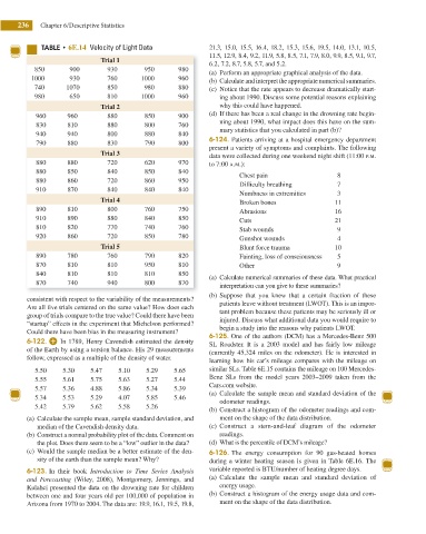
Trial 1
6.2, 7.2, 8.7, 5.8, 5.7, and 5.2.
850 900 930 950 980
(a) Perform an appropriate graphical analysis of the data.
1000 930 760 1000 960 (b) Calculate and interpret the appropriate numerical summaries.
740 1070 850 980 880 (c) Notice that the rate appears to decrease dramatically start-
980 650 810 1000 960 ing about 1990. Discuss some potential reasons explaining
Trial 2 why this could have happened.
960 960 880 850 900 (d) If there has been a real change in the drowning rate begin-
ning about 1990, what impact does this have on the sum-
830 810 880 800 760
mary statistics that you calculated in part (b)?
940 940 800 880 840
6-124. Patients arriving at a hospital emergency department
790 880 830 790 800
present a variety of symptoms and complaints. The following
Trial 3 data were collected during one weekend night shift (11:00 p.m.
880 880 720 620 970 to 7:00 a.m.):
880 850 840 850 840
Chest pain 8
880 860 720 860 950

Dificulty breathing 7
910 870 840 840 840
Numbness in extremities 3
Trial 4 Broken bones 11
890 810 800 760 750 Abrasions 16
910 890 880 840 850 Cuts 21
810 820 770 740 760 Stab wounds 9
920 860 720 850 780
Gunshot wounds 4
Trial 5 Blunt force trauma 10
890 780 760 790 820 Fainting, loss of consciousness 5
870 810 810 950 810 Other 9
840 810 810 810 850
(a) Calculate numerical summaries of these data. What practical
870 740 940 800 870
interpretation can you give to these summaries?
(b) Suppose that you knew that a certain fraction of these
consistent with respect to the variability of the measurements?
patients leave without treatment (LWOT). This is an impor-

Are all ive trials centered on the same value? How does each
tant problem because these patients may be seriously ill or
group of trials compare to the true value? Could there have been
injured. Discuss what additional data you would require to
“startup” effects in the experiment that Michelson performed?
begin a study into the reasons why patients LWOT.
Could there have been bias in the measuring instrument?
6-125. One of the authors (DCM) has a Mercedes-Benz 500
6-122. In 1789, Henry Cavendish estimated the density
SL Roadster. It is a 2003 model and has fairly low mileage
of the Earth by using a torsion balance. His 29 measurements
(currently 45,324 miles on the odometer). He is interested in
follow, expressed as a multiple of the density of water.
learning how his car’s mileage compares with the mileage on
5.50 5.30 5.47 5.10 5.29 5.65 similar SLs. Table 6E.15 contains the mileage on 100 Mercedes-
Benz SLs from the model years 2003−2009 taken from the
5.55 5.61 5.75 5.63 5.27 5.44
Cars.com website.
5.57 5.36 4.88 5.86 5.34 5.39
(a) Calculate the sample mean and standard deviation of the
5.34 5.53 5.29 4.07 5.85 5.46
odometer readings.
5.42 5.79 5.62 5.58 5.26
(b) Construct a histogram of the odometer readings and com-
(a) Calculate the sample mean, sample standard deviation, and ment on the shape of the data distribution.
median of the Cavendish density data. (c) Construct a stem-and-leaf diagram of the odometer
(b) Construct a normal probability plot of the data. Comment on readings.
the plot. Does there seem to be a “low” outlier in the data? (d) What is the percentile of DCM’s mileage?
(c) Would the sample median be a better estimate of the den- 6-126. The energy consumption for 90 gas-heated homes
sity of the earth than the sample mean? Why? during a winter heating season is given in Table 6E.16. The
6-123. In their book Introduction to Time Series Analysis variable reported is BTU/number of heating degree days.
and Forecasting (Wiley, 2008), Montgomery, Jennings, and (a) Calculate the sample mean and standard deviation of
Kulahci presented the data on the drowning rate for children energy usage.
between one and four years old per 100,000 of population in (b) Construct a histogram of the energy usage data and com-
Arizona from 1970 to 2004. The data are: 19.9, 16.1, 19.5, 19.8, ment on the shape of the data distribution.