Page 257 - Applied statistics and probability for engineers

Section 6-7/Probability Plots 235

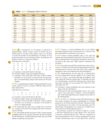
5 6E.13 Champagne Sales in France
Month 1962 1963 1964 1965 1966 1967 1968 1969
Jan. 2.851 2.541 3.113 5.375 3.633 4.016 2.639 3.934
Feb. 2.672 2.475 3.006 3.088 4.292 3.957 2.899 3.162
Mar. 2.755 3.031 4.047 3.718 4.154 4.510 3.370 4.286
Apr. 2.721 3.266 3.523 4.514 4.121 4.276 3.740 4.676
May 2.946 3.776 3.937 4.520 4.647 4.968 2.927 5.010
June 3.036 3.230 3.986 4.539 4.753 4.677 3.986 4.874
July 2.282 3.028 3.260 3.663 3.965 3.523 4.217 4.633
Aug. 2.212 1.759 1.573 1.643 1.723 1.821 1.738 1.659
Sept. 2.922 3.595 3.528 4.739 5.048 5.222 5.221 5.591
Oct. 4.301 4.474 5.211 5.428 6.922 6.873 6.424 6.981
Nov. 5.764 6.838 7.614 8.314 9.858 10.803 9.842 9.851
Dec. 7.132 8.357 9.254 10.651 11.331 13.916 13.076 12.670

6-113. A manufacturer of coil springs is interested in 6-117. Construct a normal probability plot of the efl uent
implementing a quality control system to monitor his pro- discharge temperature data from Exercise 6-112. Based on the
duction process. As part of this quality system, it is decided plot, what tentative conclusions can you draw?
to record the number of nonconforming coil springs in each 6-118. Construct normal probability plots of the cold start
production batch of size 50. During 40 days of production, 40 ignition time data presented in Exercises 6-69 and 6-80. Con-
batches of data were collected as follows: struct a separate plot for each gasoline formulation, but arrange
Read data across and down. the plots on the same axes. What tentative conclusions can
9 12 6 9 7 14 12 4 6 7 you draw?
8 5 9 7 8 11 3 6 7 7 6-119. Reconsider the golf ball overall distance data in Exer-
11 4 4 8 7 5 6 4 5 8 cise 6-41. Construct a box plot of the yardage distance and write
19 19 18 12 11 17 15 17 13 13 an interpretation of the plot. How does the box plot compare in
(a) Construct a stem-and-leaf plot of the data. interpretive value to the original stem-and-leaf diagram?
(b) Find the sample average and standard deviation. 6-120. Transformations. In some data sets, a transformation
(c) Construct a time series plot of the data. Is there evidence by some mathematical function applied to the original data,
that there was an increase or decrease in the average num- such as y or log y, can result in data that are simpler to work
ber of nonconforming springs made during the 40 days? with statistically than the original data. To illustrate the effect
Explain. of a transformation, consider the following data, which repre-
sent cycles to failure for a yarn product: 675, 3650, 175, 1150,
6-114. A communication channel is being monitored by record-
290, 2000, 100, 375.
ing the number of errors in a string of 1000 bits. Data for 20 of
(a) Construct a normal probability plot and comment on the
these strings follow:
shape of the data distribution.
Read data across and down ∗
(b) Transform the data using logarithms; that is, let y (new
3 1 0 1 3 2 4 1 3 1 value) = log (old value). Construct a normal probability
y
1 1 2 3 3 2 0 2 0 1 plot of the transformed data and comment on the effect of
(a) Construct a stem-and-leaf plot of the data. the transformation.
(b) Find the sample average and standard deviation. 6-121. In 1879, A. A. Michelson made 100 determinations of
(c) Construct a time series plot of the data. Is there evidence the velocity of light in air using a modii cation of a method
that there was an increase or decrease in the number of proposed by the French physicist Foucault. Michelson made
errors in a string? Explain. the measurements in ive trials of 20 measurements each. The

6-115. Reconsider the golf course yardage data in Exercise observations (in kilometers per second) are in Table 6E.14.
6-9. Construct a box plot of the yardages and write an interpre- Each value has 299,000 subtracted from it.
tation of the plot. The currently accepted true velocity of light in a vacuum
6-116. Reconsider the data in Exercise 6-108. Construct normal is 299,792.5 kilometers per second. Stigler (1977, The Annals
probability plots for two groups of the data: the i rst 40 and the of Statistics) reported that the “true” value for comparison to
last 40 observations. Construct both plots on the same axes. What these measurements is 734.5. Construct comparative box plots
tentative conclusions can you draw? of these measurements. Does it seem that all i ve trials are