Page 255 - Applied statistics and probability for engineers

Section 6-7/Probability Plots 233

6-99. Construct a normal probability plot of the cycles populations have the same variance, the two normal probabil-
to failure data in Exercise 6-31. Does it seem reasonable to ity plots should have identical slopes. What conclusions would
assume that cycles to failure is normally distributed? you draw about the heights of the two groups of students from
6-100. Construct a normal probability plot of the suspended visual examination of the normal probability plots?
solids concentration data in Exercise 6-40. Does it seem rea- 6-102. It is possible to obtain a “quick-and-dirty” estimate
sonable to assume that the concentration of suspended solids of the mean of a normal distribution from the 50th percentile
in water from this particular lake is normally distributed? value on a normal probability plot. Provide an argument why
6-101. Construct two normal probability plots for the height this is so. It is also possible to obtain an estimate of the stand-
data in Exercises 6-38 and 6-45. Plot the data for female ard deviation of a normal distribution by subtracting the 84th
and male students on the same axes. Does height seem to percentile value from the 50th percentile value. Provide an
be normally distributed for either group of students? If both argument explaining why this is so.

Supplemental Exercises

Problem available in WileyPLUS at instructor’s discretion.
Tutoring problem available in WileyPLUS at instructor’s discretion.
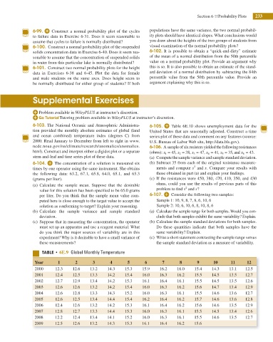
6-103. The National Oceanic and Atmospheric Administra- 6-105. Table 6E.10 shows unemployment data for the
tion provided the monthly absolute estimates of global (land United States that are seasonally adjusted. Construct a time
and ocean combined) temperature index (degrees C) from series plot of these data and comment on any features (source:
2000. Read January to December from left to right in www. U.S. Bureau of Labor Web site, http://data.bls.gov).
ncdc.noaa.gov/oa/climate/research/anomalies/anomalies. 6-106. A sample of six resistors yielded the following resistances
html). Construct and interpret either a digidot plot or a separate (ohms): x 1 = 45 , x 2 = 38 , x 3 = 47 , x 4 = 41 , x 5 = 35 , and x 6 = 43.
stem-and-leaf and time series plot of these data. (a) Compute the sample variance and sample standard deviation.
6-104. The concentration of a solution is measured six (b) Subtract 35 from each of the original resistance measure-
times by one operator using the same instrument. She obtains ments and compute s 2 and s. Compare your results with
the following data: 63.2, 67.1, 65.8, 64.0, 65.1, and 65.3 those obtained in part (a) and explain your i ndings.
(grams per liter). (c) If the resistances were 450, 380, 470, 410, 350, and 430
(a) Calculate the sample mean. Suppose that the desirable ohms, could you use the results of previous parts of this
2
value for this solution has been specii ed to be 65.0 grams problem to i nd s and s?
per liter. Do you think that the sample mean value com- 6-107. Consider the following two samples:
puted here is close enough to the target value to accept the Sample 1: 10, 9, 8, 7, 8, 6, 10, 6
solution as conforming to target? Explain your reasoning. Sample 2: 10, 6, 10, 6, 8, 10, 8, 6
(b) Calculate the sample variance and sample standard (a) Calculate the sample range for both samples. Would you con-
deviation. clude that both samples exhibit the same variability? Explain.
(c) Suppose that in measuring the concentration, the operator (b) Calculate the sample standard deviations for both samples.
must set up an apparatus and use a reagent material. What Do these quantities indicate that both samples have the
do you think the major sources of variability are in this same variability? Explain.
experiment? Why is it desirable to have a small variance of (c) Write a short statement contrasting the sample range versus
these measurements? the sample standard deviation as a measure of variability.

5"#-& t 6E.9 Global Monthly Temperature
Year 1 2 3 4 5 6 7 8 9 10 11 12
2000 12.3 12.6 13.2 14.3 15.3 15.9 16.2 16.0 15.4 14.3 13.1 12.5
2001 12.4 12.5 13.3 14.2 15.4 16.0 16.3 16.2 15.5 14.5 13.5 12.7
2002 12.7 12.9 13.4 14.2 15.3 16.1 16.4 16.1 15.5 14.5 13.5 12.6
2003 12.6 12.6 13.2 14.2 15.4 16.0 16.3 16.2 15.6 14.7 13.4 12.9
2004 12.6 12.8 13.3 14.3 15.2 16.0 16.3 16.1 15.5 14.6 13.6 12.7
2005 12.6 12.5 13.4 14.4 15.4 16.2 16.4 16.2 15.7 14.6 13.6 12.8
2006 12.4 12.6 13.2 14.2 15.3 16.1 16.4 16.2 15.6 14.6 13.5 12.9
2007 12.8 12.7 13.3 14.4 15.3 16.0 16.3 16.1 15.5 14.5 13.4 12.6
2008 12.2 12.4 13.4 14.1 15.2 16.0 16.3 16.1 15.5 14.6 13.5 12.7
2009 12.5 12.6 13.2 14.3 15.3 16.1 16.4 16.2 15.6