Page 251 - Applied statistics and probability for engineers

Section 6-6/Scatter Diagrams 229

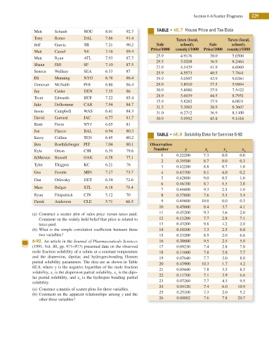
Matt Schaub HOU 8.01 92.7 5"#-& t 6E.7 House Price and Tax Data
Tony Romo DAL 7.66 91.4 Taxes (local, Taxes (local,
Jeff Garcia TB 7.21 90.2 Sale school), Sale school),
Price/1000 county)/1000 Price/1000 county)/1000
Matt Cassel NE 7.16 89.4
25.9 4.9176 30.0 5.0500
Matt Ryan ATL 7.93 87.7
29.5 5.0208 36.9 8.2464
Shaun Hill SF 7.10 87.5
27.9 4.5429 41.9 6.6969
Seneca Wallace SEA 6.33 87 25.9 4.5573 40.5 7.7841
Eli Manning NYG 6.76 86.4 29.9 5.0597 43.9 9.0384
Donovan McNabb PHI 6.86 86.4 29.9 3.8910 37.5 5.9894
Jay Cutler DEN 7.35 86 30.9 5.8980 37.9 7.5422
28.9 5.6039 44.5 8.7951
Trent Edwards BUF 7.22 85.4
35.9 5.8282 37.9 6.0831
Jake Delhomme CAR 7.94 84.7
31.5 5.3003 38.9 8.3607
Jason Campbell WAS 6.41 84.3
31.0 6.2712 36.9 8.1400
David Garrard JAC 6.77 81.7 30.9 5.9592 45.8 9.1416
Brett Favre NYJ 6.65 81
Joe Flacco BAL 6.94 80.3
5 6E.8 Solubility Data for Exercise 6-93
Kerry Collins TEN 6.45 80.2
Ben Roethlisberger PIT 7.04 80.1 Observation
Number y x x x
Kyle Orton CHI 6.39 79.6 1 2 3
1 0.22200 7.3 0.0 0.0
JaMarcus Russell OAK 6.58 77.1
2 0.39500 8.7 0.0 0.3
Tyler Thigpen KC 6.21 76
3 0.42200 8.8 0.7 1.0
Gus Freotte MIN 7.17 73.7 4 0.43700 8.1 4.0 0.2
Dan Orlovsky DET 6.34 72.6 5 0.42800 9.0 0.5 1.0
6 0.46700 8.7 1.5 2.8
Marc Bulger STL 6.18 71.4
7 0.44400 9.3 2.1 1.0
Ryan Fitzpatrick CIN 5.12 70 8 0.37800 7.6 5.1 3.4
Derek Anderson CLE 5.71 66.5 9 0.49400 10.0 0.0 0.3
10 0.45600 8.4 3.7 4.1
11 0.45200 9.3 3.6 2.0
(a) Construct a scatter plot of sales price versus taxes paid.
Comment on the widely held belief that price is related to 12 0.11200 7.7 2.8 7.1
taxes paid. 13 0.43200 9.8 4.2 2.0
(b) What is the simple correlation coefi cient between these 14 0.10100 7.3 2.5 6.8
two variables? 15 0.23200 8.5 2.0 6.6
6-92. An article in the Journal of Pharmaceuticals Sciences 16 0.30600 9.5 2.5 5.0
(1991, Vol. 80, pp. 971–977) presented data on the observed 17 0.09230 7.4 2.8 7.8
mole fraction solubility of a solute at a constant temperature 18 0.11600 7.8 2.8 7.7
and the dispersion, dipolar, and hydrogen-bonding Hansen 19 0.07640 7.7 3.0 8.0
partial solubility parameters. The data are as shown in Table
20 0.43900 10.3 1.7 4.2
6E.8, where y is the negative logarithm of the mole fraction
21 0.09440 7.8 3.3 8.5
solubility, x is the dispersion partial solubility, x is the dipo-
1 2 22 0.11700 7.1 3.9 6.6
lar partial solubility, and x is the hydrogen bonding partial
3
solubility. 23 0.07260 7.7 4.3 9.5
24 0.04120 7.4 6.0 10.9
(a) Construct a matrix of scatter plots for these variables.
25 0.25100 7.3 2.0 5.2
(b) Comment on the apparent relationships among y and the
other three variables? 26 0.00002 7.6 7.8 20.7