Page 249 - Applied statistics and probability for engineers

Section 6-6/Scatter Diagrams 227

between quality and color may exist. We saw an example of a three-dimensional scatter diagram
in Chapter 1 where we plotted wire bond strength versus wire length and die height for the bond
pull strength data.
When two or more variables exist, the matrix of scatter diagrams may be useful in
looking at all of the pairwise relationships between the variables in the sample. Figure 6-20
is the matrix of scatter diagrams (upper half only shown) for the wine quality data in
Table 6-5. The top row of the graph contains individual scatter diagrams of quality ver-
sus the other four descriptive variables, and other cells contain other pairwise plots of
the four descriptive variables pH, SO , color density, and color. This display indicates a
2
weak potential linear relationship between quality and pH and somewhat stronger potential
relationships between quality and color density and quality and color (which was noted
previously in Figure 6-19). A strong apparent linear relationship between color density and
color exists (this should be expected).
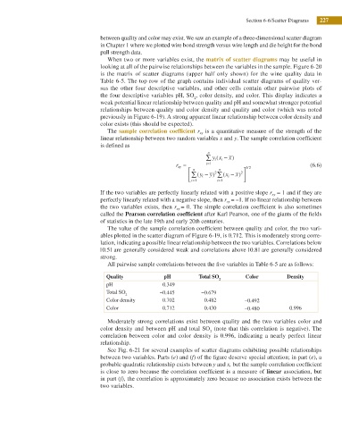
The sample correlation coeficient r xy is a quantitative measure of the strength of the
linear relationship between two random variables x and y. The sample correlation coeficient
is deined as
n
∑ y x i − )
x
i (
r xy = i=1 / 1 2 (6.6)
⎡ n 2 n 2 ⎤
x
y ∑ (
⎢ ∑ ( y i − ) x i − ) ⎥
i ⎣ =1 i=1 ⎦
If the two variables are perfectly linearly related with a positive slope r xy = 1 and if they are
perfectly linearly related with a negative slope, then r xy = −1. If no linear relationship between
= 0. The simple correlation coeficient is also sometimes
the two variables exists, then r xy
called the Pearson correlation coeficient after Karl Pearson, one of the giants of the ields
of statistics in the late 19th and early 20th centuries.
The value of the sample correlation coeficient between quality and color, the two vari-
ables plotted in the scatter diagram of Figure 6-19, is 0.712. This is moderately strong corre-
lation, indicating a possible linear relationship between the two variables. Correlations below
| 0.5 | are generally considered weak and correlations above | 0.8 | are generally considered
strong.
All pairwise sample correlations between the ive variables in Table 6-5 are as follows:
Quality pH Total SO Color Density
2
pH 0.349
Total SO −0.445 −0.679
2
Color density 0.702 0.482 −0.492
Color 0.712 0.430 −0.480 0.996

Moderately strong correlations exist between quality and the two variables color and
color density and between pH and total SO (note that this correlation is negative). The
2
correlation between color and color density is 0.996, indicating a nearly perfect linear
relationship.
See Fig. 6-21 for several examples of scatter diagrams exhibiting possible relationships
between two variables. Parts (e) and (f) of the igure deserve special attention; in part (e), a
probable quadratic relationship exists between y and x, but the sample correlation coeficient
is close to zero because the correlation coeficient is a measure of linear association, but
in part (f), the correlation is approximately zero because no association exists between the
two variables.