Page 254 - Applied statistics and probability for engineers

232 Chapter 6/Descriptive Statistics

3.30 3.30 3.30

1.65 1.65 1.65

z j 0 z j 0 z j 0

–1.65 –1.65 –1.65

–3.30 –3.30 –3.30
170 180 190 200 210 220 170 180 190 200 210 220 170 180 190 200 210 220
x ( j) x ( j) x ( j)
(a) (b) (c)
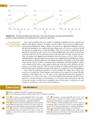
FIGURE 6-24 Normal probability plots indicating a nonnormal distribution. (a) Light-tailed distribution.
(b) Heavy-tailed distribution. (c) A distribution with positive (or right) skew.

Normal Probability The normal probability plot can be useful in identifying distributions that are symmetric but
Plots of Small Samples that have tails that are “heavier” or “lighter” than the normal. They can also be useful in iden-
Can Be Unreliable tifying skewed distributions. When a sample is selected from a light-tailed distribution (such as
the uniform distribution), the smallest and largest observations will not be as extreme as would
be expected in a sample from a normal distribution. Thus, if we consider the straight line drawn
through the observations at the center of the normal probability plot, observations on the left side
will tend to fall below the line, and observations on the right side will tend to fall above the line.
This will produce an S-shaped normal probability plot such as shown in Fig. 6-24(a). A heavy-
tailed distribution will result in data that also produce an S-shaped normal probability plot, but now
the observations on the left will be above the straight line and the observations on the right will lie
below the line. See Fig. 6-24(b). A positively skewed distribution will tend to produce a pattern
such as shown in Fig. 6-24(c), where points on both ends of the plot tend to fall below the line,
giving a curved shape to the plot. This occurs because both the smallest and the largest observa-
tions from this type of distribution are larger than expected in a sample from a normal distribution.
Even when the underlying population is exactly normal, the sample data will not plot
exactly on a straight line. Some judgment and experience are required to evaluate the plot.
Generally, if the sample size is n < 30, there can be signiicant deviation from linearity in
normal plots, so in these cases only a very severe departure from linearity should be inter-
preted as a strong indication of nonnormality. As n increases, the linear pattern will tend
to become stronger, and the normal probability plot will be easier to interpret and more
reliable as an indicator of the form of the distribution.

Exercises FOR SECTION 6-7

Problem available in WileyPLUS at instructor’s discretion.
Tutoring problem available in WileyPLUS at instructor’s discretion.
6-93. Construct a normal probability plot of the piston 6-96. Construct a normal probability plot of the solar
ring diameter data in Exercise 6-7. Does it seem reasonable to intensity data in Exercise 6-12. Does it seem reasonable to
assume that piston ring diameter is normally distributed? assume that solar intensity is normally distributed?
6-94. Construct a normal probability plot of the insulating 6-97. Construct a normal probability plot of the O-ring joint
luid breakdown time data in Exercise 6-8. Does it seem rea- temperature data in Exercise 6-19. Does it seem reasonable to
sonable to assume that breakdown time is normally distributed? assume that O-ring joint temperature is normally distributed?
6-95. Construct a normal probability plot of the visual Discuss any interesting features that you see on the plot.
accommodation data in Exercise 6-11. Does it seem rea- 6-98. Construct a normal probability plot of the octane
sonable to assume that visual accommodation is normally rating data in Exercise 6-30. Does it seem reasonable to assume
distributed? that octane rating is normally distributed?