Page 256 - Applied statistics and probability for engineers

234 Chapter 6/Descriptive Statistics

5"#-& t 6E.10 Unemployment Percentage
Year Jan Feb Mar Apr May Jun Jul Aug Sep Oct Nov Dec
1999 4.3 4.4 4.2 4.3 4.2 4.3 4.3 4.2 4.2 4.1 4.1 4.0
2000 4.0 4.1 4.0 3.8 4.0 4.0 4.0 4.1 3.9 3.9 3.9 3.9
2001 4.2 4.2 4.3 4.4 4.3 4.5 4.6 4.9 5.0 5.3 5.5 5.7
2002 5.7 5.7 5.7 5.9 5.8 5.8 5.8 5.7 5.7 5.7 5.9 6.0
2003 5.8 5.9 5.9 6.0 6.1 6.3 6.2 6.1 6.1 6.0 5.8 5.7
2004 5.7 5.6 5.8 5.6 5.6 5.6 5.5 5.4 5.4 5.5 5.4 5.4
2005 5.2 5.4 5.2 5.2 5.1 5.1 5.0 4.9 5.0 5.0 5.0 4.8
2006 4.7 4.8 4.7 4.7 4.7 4.6 4.7 4.7 4.5 4.4 4.5 4.4
2007 4.6 4.5 4.4 4.5 4.5 4.6 4.7 4.7 4.7 4.8 4.7 4.9
2008 4.9 4.8 5.1 5.0 5.5 5.6 5.8 6.2 6.2 6.6 6.8 7.2
2009 7.6 8.1 8.5 8.9 9.4 9.5 9.4 9.7 9.8

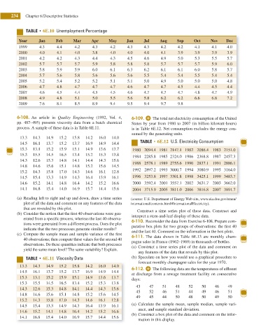
6-108. An article in Quality Engineering (1992, Vol. 4, 6-109. The total net electricity consumption of the United
pp. 487–495) presents viscosity data from a batch chemical States by year from 1980 to 2007 (in billion kilowatt-hours)
process. A sample of these data is in Table 6E.11. is in Table 6E.12. Net consumption excludes the energy con-
sumed by the generating units.
13.3 14.3 14.9 15.2 15.8 14.2 16.0 14.0
TABLE t 6E.12 U.S. Electricity Consumption
14.5 16.1 13.7 15.2 13.7 16.9 14.9 14.4
15.3 13.1 15.2 15.9 15.1 14.9 13.6 13.7 1980 2094.4 1981 2147.1 1982 2086.4 1983 2151.0
15.3 15.5 14.5 16.5 13.4 15.2 15.3 13.8
1984 2285.8 1985 2324.0 1986 2368.8 1987 2457.3
14.3 12.6 15.3 14.8 14.1 14.4 14.3 15.6
1988 2578.1 1989 2755.6 1990 2837.1 1991 2886.1
14.8 14.6 15.6 15.1 14.8 15.2 15.6 14.5
1992 2897.2 1993 3000.7 1994 3080.9 1995 3164.0
15.2 14.3 15.8 17.0 14.3 14.6 16.1 12.8
14.5 15.4 13.3 14.9 14.3 16.4 13.9 16.1 1996 3253.8 1997 3301.8 1998 3425.1 1999 3483.7
14.6 15.2 14.1 14.8 16.4 14.2 15.2 16.6 2000 3592.4 2001 3557.1 2002 3631.7 2003 3662.0
14.1 16.8 15.4 14.0 16.9 15.7 14.4 15.6 2004 3715.9 2005 3811.0 2006 3816.8 2007 3891.7

(a) Reading left to right and up and down, draw a time series (source: U.S. Department of Energy Web site, www.eia.doe.gov/emeu/
plot of all the data and comment on any features of the data international/contents.html#InternationalElectricity).
that are revealed by this plot.
Construct a time series plot of these data. Construct and
(b) Consider the notion that the irst 40 observations were gen-

interpret a stem-and-leaf display of these data.
erated from a speciic process, whereas the last 40 observa-

6-110. Reconsider the data from Exercise 6-108. Prepare com-
tions were generated from a different process. Does the plot
parative box plots for two groups of observations: the i rst 40
indicate that the two processes generate similar results?
and the last 40. Comment on the information in the box plots.
(c) Compute the sample mean and sample variance of the i rst
6-111. The data shown in Table 6E.13 are monthly cham-
40 observations; then compute these values for the second 40
pagne sales in France (1962–1969) in thousands of bottles.
observations. Do these quantities indicate that both processes
(a) Construct a time series plot of the data and comment on
yield the same mean level? The same variability? Explain.
any features of the data that reveals by this plot.
5"#-& t 6E.11 Viscosity Data (b) Speculate on how you would use a graphical procedure to
forecast monthly champagne sales for the year 1970.
13.3 14.3 14.9 15.2 15.8 14.2 16.0 14.0
6-112. The following data are the temperatures of efl uent
14.5 16.1 13.7 15.2 13.7 16.9 14.9 14.4
at discharge from a sewage treatment facility on consecutive
15.3 13.1 15.2 15.9 15.1 14.9 13.6 13.7
days:
15.3 15.5 14.5 16.5 13.4 15.2 15.3 13.8
43 47 51 48 52 50 46 49
14.3 12.6 15.3 14.8 14.1 14.4 14.3 15.6
45 52 46 51 44 49 46 51
14.8 14.6 15.6 15.1 14.8 15.2 15.6 14.5
49 45 44 50 48 50 49 50
15.2 14.3 15.8 17.0 14.3 14.6 16.1 12.8
14.5 15.4 13.3 14.9 14.3 16.4 13.9 16.1 (a) Calculate the sample mean, sample median, sample vari-
ance, and sample standard deviation.
14.6 15.2 14.1 14.8 16.4 14.2 15.2 16.6
(b) Construct a box plot of the data and comment on the infor-
14.1 16.8 15.4 14.0 16.9 15.7 14.4 15.6
mation in this display.