Page 34 - Applied statistics and probability for engineers

12 Chapter 1/The Role of Statistics in Engineering

where the β’s are unknown parameters. Now just as in Ohm’s law, this model will not exactly
describe the phenomenon, so we should account for the other sources of variability that may
affect the molecular weight by adding another term to the model; therefore,
M n = β + β 1 V + β 2 C + β 3 T + e (1-6)
0
is the model that we will use to relate molecular weight to the other three variables. This
type of model is called an empirical model; that is, it uses our engineering and scientiic
knowledge of the phenomenon, but it is not directly developed from our theoretical or irst-
principles understanding of the underlying mechanism.
To illustrate these ideas with a speciic example, consider the data in Table 1-2, which contains
data on three variables that were collected in an observational study in a semiconductor manu-
facturing plant. In this plant, the inished semiconductor is wire-bonded to a frame. The variables
reported are pull strength (a measure of the amount of force required to break the bond), the wire
length, and the height of the die. We would like to ind a model relating pull strength to wire length
and die height. Unfortunately, there is no physical mechanism that we can easily apply here, so it
does not seem likely that a mechanistic modeling approach will be successful.
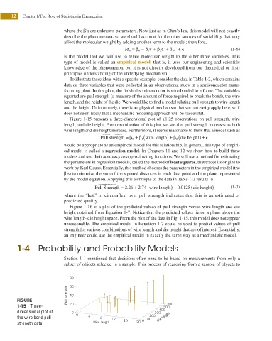
Figure 1-15 presents a three-dimensional plot of all 25 observations on pull strength, wire
length, and die height. From examination of this plot, we see that pull strength increases as both
wire length and die height increase. Furthermore, it seems reasonable to think that a model such as
)

Pull strength = β + β 1( wire length + β 2( die height + ) e
0
would be appropriate as an empirical model for this relationship. In general, this type of empiri-
cal model is called a regression model. In Chapters 11 and 12 we show how to build these
models and test their adequacy as approximating functions. We will use a method for estimating
the parameters in regression models, called the method of least squares, that traces its origins to
work by Karl Gauss. Essentially, this method chooses the parameters in the empirical model (the
β’s) to minimize the sum of the squared distances in each data point and the plane represented
by the model equation. Applying this technique to the data in Table 1-2 results in

Pull Strength = 2 26 + 2 74 ( wire length) + 0 0125 ( die height) (1-7)
.
.
.
where the “hat,” or circum8x, over pull strength indicates that this is an estimated or
predicted quality.
Figure 1-16 is a plot of the predicted values of pull strength versus wire length and die
height obtained from Equation 1-7. Notice that the predicted values lie on a plane above the
wire length–die height space. From the plot of the data in Fig. 1-15, this model does not appear
unreasonable. The empirical model in Equation 1-7 could be used to predict values of pull
strength for various combinations of wire length and die height that are of interest. Essentially,
an engineer could use the empirical model in exactly the same way as a mechanistic model.

1-4 Probability and Probability Models

Section 1-1 mentioned that decisions often need to be based on measurements from only a
subset of objects selected in a sample. This process of reasoning from a sample of objects to

80

Pull strength 60 40

FIGURE
600
1-15 Three- 20 500
dimensional plot of 0 300 400
the wire bond pull 0 4 8 12 100 200 Die height
strength data. Wire length 16 20 0