Page 31 - Applied statistics and probability for engineers

Section 1-2/Collecting Engineering Data 9

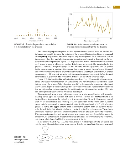
100
Acetone concentration 90

80
x
80.5 84.0 87.5 91.0 94.5 98.0 10 20 30
Acetone concentration Observation number (hour)
FIGURE 1-8 The dot diagram illustrates variation FIGURE 1-9 A time series plot of concentration
but does not identify the problem. provides more information than the dot diagram.
This interesting experiment points out that adjustments to a process based on random dis-
turbances can actually increase the variation of the process. This is referred to as overcontrol
or tampering. Adjustments should be applied only to compensate for a nonrandom shift in
the process—then they can help. A computer simulation can be used to demonstrate the les-
sons of the funnel experiment. Figure 1-11 displays a time plot of 100 measurements (denoted
as y) from a process in which only random disturbances are present. The target value for the
process is 10 units. The igure displays the data with and without adjustments that are applied
to the process mean in an attempt to produce data closer to target. Each adjustment is equal
and opposite to the deviation of the previous measurement from target. For example, when the
measurement is 11 (one unit above target), the mean is reduced by one unit before the next
measurement is generated. The overcontrol increases the deviations from the target.
Figure 1-12 displays the data without adjustment from Fig. 1-11, except that the measure-
ments after observation number 50 are increased by two units to simulate the effect of a shift
in the mean of the process. When there is a true shift in the mean of a process, an adjustment
can be useful. Figure 1-12 also displays the data obtained when one adjustment (a decrease of
two units) is applied to the mean after the shift is detected (at observation number 57). Note
that this adjustment decreases the deviations from target.
The question of when to apply adjustments (and by what amounts) begins with an under-
standing of the types of variation that affect a process. The use of a control charts is an
invaluable way to examine the variability in time-oriented data. Figure 1-13 presents a control
chart for the concentration data from Fig. 1-9. The center line on the control chart is just the
/
average of the concentration measurements for the irst 20 samples (x = 91.5 g l) when the
process is stable. The upper control limit and the lower control limit are a pair of statisti-
cally derived limits that relect the inherent or natural variability in the process. These limits
are located 3 standard deviations of the concentration values above and below the center line.
If the process is operating as it should without any external sources of variability present in
the system, the concentration measurements should luctuate randomly around the center line,
and almost all of them should fall between the control limits.
In the control chart of Fig. 1-13, the visual frame of reference provided by the center line
and the control limits indicates that some upset or disturbance has affected the process around

FIGURE 1-10
Deming’s funnel
experiment. Target Marbles