Page 166 - Applied Statistics Using SPSS, STATISTICA, MATLAB and R

146 4 Parametric Tests of Hypotheses

In the configuration of Figure 4.13b (null hypothesis is false), the between-
group variance no longer represents an estimate of the population variance. In this
case, we obtain a ratio v B/v W larger than 1. (In this case the contribution of v B to the
final value of v in 4.30 is smaller than the contribution of v W.)
The one-way ANOVA, assuming the test conditions are satisfied, uses the
following test statistic (see properties of the F distribution in section B.2.9):

v MSB
*
F = B = ~ F c− , n− c (under H 0). 4.33
1
v W MSE

*
If H 0 is not true, then F exceeds 1 in a statistically significant way.
The F distribution can be used even when there are mild deviations from the
assumptions of normality and equality of variances. The equality of variances can
be assessed using the ANOVA generalization of Levene’s test described in the
section 4.4.2.2.

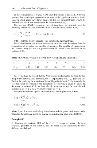
Table 4.9. Critical F values at α = 0.05 for n = 25 and several values of c.
c 2 3 4 5 6 7 8

F c−1,n−c 4.26 3.42 3.05 2.84 2.71 2.63 2.58

For c = 2, it can be proved that the ANOVA test is identical to the t test for two
independent samples. As c increases, the 1 – α percentile of F c−1,n−c decreases (see
Table 4.9), rendering the rejection of the null hypothesis “easier”. Equivalently, for
*
a certain level of confidence the probability of observing a given F under H 0
decreases. In section 4.5.1, we have already made use of the fact that the null
c
c
hypothesis for > 2 is more “restrictive” than for = 2.
The previous sums of squares can be shown to be computable as follows:

c r i
2
n
SST = ∑∑ x ij 2 −T / , 4.34a
= i 1 = j 1
c
2
2
SSB = ∑ ( T / r ) −T / , 4.34b
n
i
i
= i 1

where T i and T are the totals along the columns and the grand total, respectively.
These last formulas are useful for manual computation (or when using EXCEL).
Example 4.13
Q: Consider the variable ART of the Cork Stoppers’ dataset. Is there
evidence, provided by the samples, that the three classes correspond to three
different populations?