Page 165 - Applied Statistics Using SPSS, STATISTICA, MATLAB and R

4.5 Inference on More than Two Populations 145

The ANOVA test uses precisely this “analysis of variance” property. Notice that
the total number of degrees of freedom, n – 1, is also broken down into two parts:
n – c and c – 1.
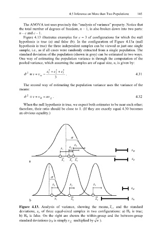
Figure 4.13 illustrates examples for c = 3 of configurations for which the null
hypothesis is true (a) and false (b). In the configuration of Figure 4.13a (null
hypothesis is true) the three independent samples can be viewed as just one single
sample, i.e., as if all cases were randomly extracted from a single population. The
standard deviation of the population (shown in grey) can be estimated in two ways.
One way of estimating the population variance is through the computation of the
pooled variance, which assuming the samples are of equal size, n, is given by:

2
2
s + s + s 2
ˆ ≡
σ 2 v ≈ v = 1 2 3 . 4.31
w
3

The second way of estimating the population variance uses the variance of the
means:
ˆ σ 2 ≡ v ≈ v = nv . 4.32
B
X
When the null hypothesis is true, we expect both estimates to be near each other;
therefore, their ratio should be close to 1. (If they are exactly equal 4.30 becomes
an obvious equality.)

σ
s 3
s 1 s 2 s W

a x 1 x x 3 s B
2

σ

s 1 s 2 s 3
s W

x x x s
b 1 2 3 B
Figure 4.13. Analysis of variance, showing the means, x , and the standard
i
deviations, s i, of three equal-sized samples in two configurations: a) H 0 is true;
b) H 0 is false. On the right are shown the within-group and the between-group
standard deviations (s B is simply s multiplied by n ).
X