Page 170 - Applied Statistics Using SPSS, STATISTICA, MATLAB and R

150 4 Parametric Tests of Hypotheses

“Post hoc” comparisons (e.g. Scheffé test), to be dealt with in the following
section, are accessible using the Post-hoc tab in STATISTICA (click More
Results ) or clicking the ost Hoc P button in SPSS. Contrasts can be performed
using the Planned comps tab in STATISTICA (click More Res ults ) or
clicking the Contrasts button in SPSS.
Note that the ANOVA commands are also used in regression analysis, as
explained in Chapter 7. When performing regression analysis, one often considers
an “intercept” factor in the model. When comparing means, this factor is
meaningless. Be sure, therefore, to check the No intercept box in
STATISTICA (Options tab) and uncheck Include intercept in the
model in SPSS ( Linear Model General ). In STATISTICA the Sigma-
restricted box must also be unchecked.
The meanings of the arguments and return values of MATLAB anova1
command are as follows:

p : p value of the null hypothesis;
table : matrix for storing the returned ANOVA table;
stats : test statistics, useful for performing multiple comparison of means
with the multcompare function;
x : data matrix with each column corresponding to an independent
sample;
group : optional character array with group names in each row;
dispopt: display option with two values, ‘on’ and ‘off’. The default ‘on’
displays plots of the results (including the ANOVA table).

We now illustrate how to apply the one-way ANOVA test in R for the Example
4.14. The first thing to do is to create the ART1 variable with ART1 <-
log(ART) . We then proceed to create a factor variable from the data frame
classification variable denoted CL . The factor variable type in R is used to define a
categorical variable with label values. The need of this step is that the ANOVA test
can also be applied to continuous variables as we will see in Chapter 7. The
creation of a factor variable from the numerical variable CL can be done with:

“
“
> CLf <- factor(CL,labels=c(“I”, II”, III”))

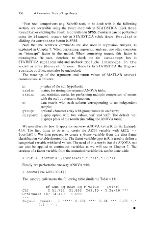
Finally, we perform the one-way ANOVA with:

> anova(lm(ART1~CLf))

The anova call returns the following table similar to Table 4.13:

Df Sum Sq Mean Sq F value Pr(>F)
CLf 2 51.732 25.866 263.15 < 2.2e-16 ***
Residuals 147 14.449 0.098
---
Signif. codes: 0 ‘***’ 0.001 ‘**’ 0.01 ‘*’ 0.05 ‘.’
0.1 ‘ 1
’