Page 174 - Applied Statistics Using SPSS, STATISTICA, MATLAB and R

154 4 Parametric Tests of Hypotheses

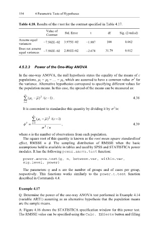
Table 4.18. Results of the t test for the contrast specified in Table 4.17.
Value of
Contrast Std. Error t df Sig. (2-tailed)
Assume equal 3.975E−02 100 0.062
variances −7.502E−02 −1.887
Does not assume 2.801E−02 31.79 0.012
equal variances −7.502E−02 −2.678

4.5.2.3 Power of the One-Way ANOVA

In the one-way ANOVA, the null hypothesis states the equality of the means of c
2
populations, µ 1 = µ 2 = … = µ c, which are assumed to have a common value σ for
the variance. Alternative hypothesies correspond to specifying different values for
the population means. In this case, the spread of the means can be measured as:

c
∑ (µ i − ) 2 /( c − ) . 4.38
µ
1
= i 1

2
It is convenient to standardise this quantity by dividing it by σ /n:

c
∑ (µ − µ ) 2 /( − )
c 1
i
2
φ = i 1 = , 4.39
σ 2 n /

where n is the number of observations from each population.
The square root of this quantity is known as the root mean square standardised
effect, RMSSE ≡ φ. The sampling distribution of RMSSE when the basic
assumptions hold is available in tables and used by SPSS and STATISTICA power
modules. R has the following power.anova.test function:

power.anova.test(g, n, between.var, within.var,
sig.level, power)

The parameters g and n are the number of groups and of cases per group,
respectively. This functions works similarly to the power.t.test function
described in Commands 4.4.

Example 4.17
Q: Determine the power of the one-way ANOVA test performed in Example 4.14
(variable ART1) assuming as an alternative hypothesis that the population means
are the sample means.

A: Figure 4.16 shows the STATISTICA specification window for this power test.
The RMSSE value can be specified using the Calc. Effects button and filling