Page 177 - Applied Statistics Using SPSS, STATISTICA, MATLAB and R

4.5 Inference on More than Two Populations 157

c r
SST = ∑∑ (x ij − x .. ) 2
1 = i 1 = j
c r c r
= ∑ (x . i − x .. ) + ∑ (x . j − x .. ) +∑∑ (x ij − x . i − x . j + x .. ) 4.40
2
2
2
r
c
1 = i 1 = j 1 = i 1 = j
= SSC + SSR + SSE .

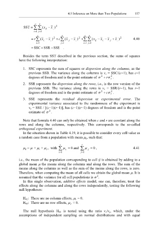
Besides the term SST described in the previous section, the sums of squares
have the following interpretation:

1. SSC represents the sum of squares or dispersion along the columns, as the
previous SSB. The variance along the columns is v c = SSC/(c−1), has c−1
2
2
degrees of freedom and is the point estimate of σ + rσ .
c
2. SSR represents the dispersion along the rows, i.e., is the row version of the
previous SSB. The variance along the rows is v r = SSR/(r−1), has r−1
2
2
degrees of freedom and is the point estimate of σ + cσ .
r
3. SSE represents the residual dispersion or experimental error. The
experimental variance associated to the randomness of the experiment is
v e = SSE / [(c−1)(r−1)], has (c−1)(r−1) degrees of freedom and is the point
2
estimate of σ .

Note that formula 4.40 can only be obtained when c and r are constant along the
rows and along the columns, respectively. This corresponds to the so-called
orthogonal experiment.
In the situation shown in Table 4.19, it is possible to consider every cell value as
a random case from a population with mean µ ij, such that:

c r
µ ij = µ + µ i. + µ .j , with ∑ µ i. = 0 and ∑ µ j . = 0 , 4.41
= i 1 = j 1

i.e., the mean of the population corresponding to cell ij is obtained by adding to a
global mean µ the means along the columns and along the rows. The sum of the
means along the columns as well as the sum of the means along the rows, is zero.
Therefore, when computing the mean of all cells we obtain the global mean µ. It is
2
assumed that the variance for all cell populations is σ .
In this single observation, additive effects model, one can, therefore, treat the
effects along the columns and along the rows independently, testing the following
null hypotheses:

H 01: There are no column effects, µ i. = 0.
H 02: There are no row effects, µ .j = 0.

The null hypothesis H 01 is tested using the ratio v c/v e, which, under the
assumptions of independent sampling on normal distributions and with equal