Page 181 - Applied Statistics Using SPSS, STATISTICA, MATLAB and R

4.5 Inference on More than Two Populations 161

Notice that in Table 4.21 the total sum of squares and the model sum of squares
are computed using formulas 4.43a and 4.43b, respectively, without the last term of
these formulas. Therefore, the degrees of freedom are crn and cr, respectively.

Table 4.21. Two-way ANOVA test results, obtained with SPSS, for Example 4.19.
Type III Sum of
Source df Mean Square F Sig.
Squares
Model 46981.250 6 7830.208 220.311 0.000
F1 108.083 2 54.042 1.521 0.245
F2 630.375 1 630.375 17.736 0.001
F1 * F2 a 217.750 2 108.875 3.063 0.072
Error 639.750 18 35.542
Total 47621.000 24
a Interaction term.

60

50

Estimated Marginal Means 40 F2 1

30
1 F1 2 3 2

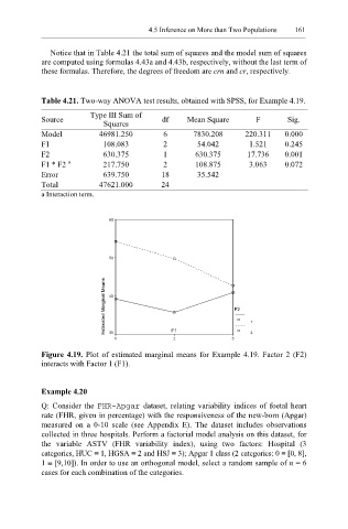
Figure 4.19. Plot of estimated marginal means for Example 4.19. Factor 2 (F2)
interacts with Factor 1 (F1).

Example 4.20

Q: Consider the FHR-Apg ar dataset, relating variability indices of foetal heart
rate (FHR, given in percentage) with the responsiveness of the new-born (Apgar)
measured on a 0-10 scale (see Appendix E). The dataset includes observations
collected in three hospitals. Perform a factorial model analysis on this dataset, for
the variable ASTV (FHR variability index), using two factors: Hospital (3
categories, HUC ≡ 1, HGSA ≡ 2 and HSJ ≡ 3); Apgar 1 class (2 categories: 0 ≡ [0, 8],
1 ≡ [9,10]). In order to use an orthogonal model, select a random sample of n = 6
cases for each combination of the categories.