Page 180 - Applied Statistics Using SPSS, STATISTICA, MATLAB and R

160 4 Parametric Tests of Hypotheses

c r
2
SSE = SST − ∑∑ ij. 2 n / −T /( rcn) , 4.43e
T
...
= i 1 = j 1

where T i.., T .j., T ij. and T ... are the totals along the columns, along the rows, in each
cell and the grand total, respectively. These last formulas are useful for manual
computation (or when using EXCEL).

Example 4.19
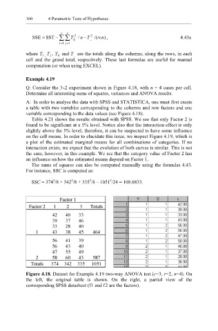
Q: Consider the 3×2 experiment shown in Figure 4.18, with n = 4 cases per cell.
Determine all interesting sums of squares, variances and ANOVA results.
A: In order to analyse the data with SPSS and STATISTICA, one must first create
a table with two variables corresponding to the columns and row factors and one
variable corresponding to the data values (see Figure 4.18).
Table 4.21 shows the results obtained with SPSS. We see that only Factor 2 is
found to be significant at a 5% level. Notice also that the interaction effect is only
slightly above the 5% level; therefore, it can be suspected to have some influence
on the cell means. In order to elucidate this issue, we inspect Figure 4.19, which is
a plot of the estimated marginal means for all combinations of categories. If no
interaction exists, we expect that the evolution of both curves is similar. This is not
the case, however, in this example. We see that the category value of Factor 2 has
an influence on how the estimated means depend on Factor 1.
The sums of squares can also be computed manually using the formulas 4.43.
For instance, SSC is computed as:

2
2
2
2
SSC = 374 /8 + 342 /8 + 335 /8 – 1051 /24 = 108.0833.

Figure 4.18. Dataset for Example 4.19 two-way ANOVA test (c=3, r=2, n=4). On
the left, the original table is shown. On the right, a partial view of the
corresponding SPSS datasheet (f1 and f2 are the factors).