Page 235 - Applied Statistics Using SPSS, STATISTICA, MATLAB and R

216 5 Non-Parametric Tests of Hypotheses

Tables with the exact probabilities of F r, under the null hypothesis, can be found
in the literature. For c > 5 or for n > 15 F r has an asymptotic chi-square distribution
with df = c – 1 degrees of freedom.
When there are tied ranks, a correction is inserted in formula 5.40, subtracting
from nc(c + 1) in the denominator the following term:

n g i
nc − ∑∑ t 3 i . j
1 = i 1 = j , 5.41
c − 1

where t i.j is the number of ties in group j of g i tied groups in the ith row.
The power-efficiency of the Friedman test, when compared with its parametric
counterpart, the two-way ANOVA, is 64% for c = 2 and increases with c, namely
to 80% for c = 5.

Example 5.24
Q: Consider the evaluation of a sample of eight metallurgic firms ( Metal
Firms’ dataset), in what concerns social impact, with variables: CEI =
“commitment to environmental issues”; IRM = “incentive towards using recyclable
materials”; EMS = “environmental management system”; CLC = “co-operation
with local community”; OEL = “obedience to environmental legislation”. Is there
evidence at a 5% level that all variables have distributions with the same median?

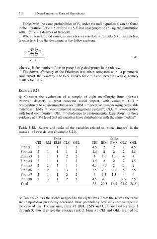
Table 5.28. Scores and ranks of the variables related to “social impact” in the
Metal Firms dataset (Example 5.24).
Data Ranks
CEI IRM EMS CLC OEL CEI IRM EMS CLC OEL
Firm #1 2 1 1 1 2 4.5 2 2 2 4.5
Firm #2 2 1 1 1 2 4.5 2 2 2 4.5
Firm #3 2 1 1 2 2 4 1.5 1.5 4 4
Firm #4 2 1 1 1 2 4.5 2 2 2 4.5
Firm #5 2 2 1 1 1 4.5 4.5 2 2 2
Firm #6 2 2 2 3 2 2.5 2.5 2.5 5 2.5
Firm #7 2 1 1 2 2 4 1.5 1.5 4 4
Firm #8 3 3 1 2 2 4.5 4.5 1 2.5 2.5
Total 33 20.5 14.5 23.5 28.5

A: Table 5.28 lists the scores assigned to the eight firms. From the scores, the ranks
are computed as previously described. Note particularly how ranks are assigned in
the case of ties. For instance, Firm #1 IRM, EMS and CLC are tied for rank 1
through 3; thus they get the average rank 2. Firm #1 CEI and OEL are tied for