Page 60 - Artificial Intelligence for Computational Modeling of the Heart

30 Chapter 1 Multi-scale models of the heart for patient-specific simulations

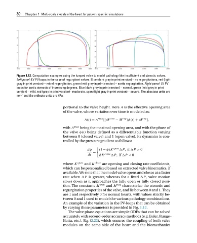
Figure 1.12. Computation examples using the lumped valve to model pathology like insufficient and stenotic valves.
Left panel: LV PV loops in the case of regurgitant valves. Blue (dark gray in print version) – no regurgitations, red (light
gray in print version) – mitral regurgitation, green (mid gray in print version) – aortic regurgitation. Right panel:LVPV
loops for aortic stenosis of increasing degrees. Blue (dark gray in print version) – normal, green (mid gray in print
version) – mild, red (gray in print version)– moderate, cyan (light gray in print version) – severe. The abscissa units are
3
mm and the ordinate units are kPa.

portional to the valve height. Here A is the effective opening area
of the valve, whose variation over time is modeled as:
A(t) = A max [(M sten − M reg )φ(t) + M reg ],

with A max being the maximal opening area, and with the phase of
the valve φ(t) being defined as a differentiable function varying
between 0 (closed valve) and 1 (open valve). Its dynamics is con-
trolled by the pressure gradient as follows:
open
dφ (1 − φ)K
P, if
P > 0
=
dt φK close
P, if
P < 0
where K open and K close are opening and closing rate coefficients,
which can be personalized based on extracted valve kinematics, if
available. We note that the model valve opens and closes at a faster
rate when
P is greater, whereas for a fixed
P, valve motion
slows down as it approaches the fully open or fully closed posi-
tion. The constants M sten and M reg characterize the stenotic and
regurgitation properties of the valve, and lie between 0 and 1. They
are 1 and respectively 0 for normal hearts, with values strictly be-
tween 0 and 1 used to model the various pathology combinations.
An example of the variation in the PV-loops that can be obtained
by varying these parameters is provided in Fig. 1.12.
The valve phase equations are simple ODEs that can be solved
accurately with second-order accuracy methods (e.g. Euler, Runge–
Kutta, etc.). Eq. (2.22), which ensures the coupling of both valve
modules on the same side of the heart and the biomechanics