Page 757 - Automotive Engineering Powertrain Chassis System and Vehicle Body

CHAP TER 2 2. 1 Exterior noise: Assessment and control

analysed, first for the engine at full load (Bosch, 1986) The method adopted here allows the intake designer
and then subsequently for part load operation, and finally to calculate intake Mach numbers using practical engine
for the engine installed in the vehicle. performance data (brake power and bsfc) with the need
The chain of efficiencies for the engine itself, operat- for only a limited set of additional data, all of which is
ing at full load throttle is given by: freely available in the literature.

h engine ¼ h h h h m (22.1.67) 22.1.3.12.13 Describing the acoustic
c
i
d
performance of flow duct systems
where
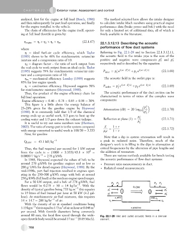
h i ¼ ideal fuel–air cycle efficiency, which Taylor Referring to Fig. 22.1-28 and to Section 22.1.3.12.11,
(1985) shows to be 46% for stoichiometric octane/air the acoustic field in the intake pipe is the sum of the
þ
mixture and a compression ratio of 10. positive and negative wave components p 1 and p 1
h d ¼ diagram factor – the ratio of work output from respectively and is described by the equation
the real cycle to work output from an ideal cycle. Taylor þ
iðutþb xÞ
þ iðut b xÞ
(1985) suggests 78% for stoichiometric octane/air mix- P inlet ¼ p e 1 þ p e 1 (22.1.68)
1
1
ture and a compression ratio of 10.
h m ¼ mechanical efficiency. Lumley (1999) suggests The acoustic field in the outlet pipe is:
85% for low engine speeds.
iðut b xÞ
þ iðut b xÞ
h c ¼ combustion efficiency. Heywood suggests 98% P outlet ¼ p e þ 2 þ p e 2 (22.1.69)
2
2
for stoichometric mixtures (Heywood, 1988).
Thus, the product of the engine efficiency chain for The acoustic performance of the duct section can be
full load operation: characterised in terms of ratios of the complex wave
Engine efficiency ¼ 0.46 0.78 0.85 0.98 ¼ 30% components:
This figure is a little above the energy balance of þ
25–28% given for the gasoline engine by Heywood Attenuation ðdBÞ¼ 20 log p 1 (22.1.70)
(1988). It is commonly held that 1/3 of the chemical 10 p þ
2
energy ends up as useful work, 1/3 goes to heat up the p
cooling water and 1/3 goes down the exhaust tailpipe. Reflection at plane ð1Þ¼ p 1 þ (22.1.71)
It is useful to try out some numbers now (Harrison, 1
2003). The ratio of energy put in to the system compared Z ¼ 1 þ r (22.1.72)
with energy converted to useful work is 100/30 ¼ 3.333 r c 1 r
0
Now, for gasoline
Note that a dip in system attenuation will result in
Q LHV ¼ 43:1MJ=kg 1 a peak in radiated noise. Therefore, much of the
designer’s work is in filling in the dips in attenuation at
Thus, the fuel required per second for 1 kW output critical frequencies by the alteration of pipe lengths and
6
from the cycle is ¼ (1000 3.333)/43.1 10 ¼ the addition of resonators.
0.000077 kg/s 1 ¼ 278 g/kWh There are various methods available for bench testing
In 1988, Heywood expected the values of bsfc to be the acoustic performance of flow duct systems:
around 270 g/kWh for gasoline engines and as low as Pressure ratio measurements in duct.
200 g/ kWh for diesel engines (Heywood, 1988). By the Radiated sound measurements.
mid-1990s, port fuel injection resulted in engines oper-
ating in the 250–300 g/kWh range with bsfc at around
250 g/kWh (full load) at the medium engine speed ranges.
For a 50 kW output, and a bsfc of 278 g/kWh, fuel P P P P
1
flows would be 0.278 50 ¼ 14 kg/hr . With the 2 1 FLOW 3 4
density of typical gasoline being 733 kg m 3 this equates p + 1 1 p 2 +
to 19 litres of fuel burned per hour at 50 kW (4.2 gal- p – 1 2 p – 2
lons). At stoichiometric air-fuel mixtures, this requires x 1 x 3
14 14.7 ¼ 206 kg/hr 1 of air. x 2 x 4
With the density of air at standard conditions being
3
1.19kgm 3 thisisequalto173m ofairanhouror0.048m 3 x positive
per second. With throttle diameters being commonly
around 60 mm, the local flow speed through the wide- Fig. 22.1-28 Inlet and outlet acoustic fields in a silencer
open throttle bodywould be around 17 ms 1 (0.05 Mach). element.

768