Page 196 - Basics of MATLAB and Beyond

We change variables:

p = C + Bx .
Now we simply do a least-squares fit using this equation; that is, a
straight line. We could use the backslash notation that we used to fit
the parabola but, for variety, let’s use the polyfit function. A straight
line is a polynomial of degree 1. The following code takes the logarithm
of the population data and fits a straight line to it:

>> logp = log(P);
>> c = polyfit(year,logp,1)
c=
0.0430 -68.2191
The vector c contains B and C, in that order. We use the polynomial
evaluation function polyval to calculate the fitted population over a fine
year grid:

>> year_fine = (year(1):0.5:year(length(year)))’;
>> logpfit = polyval(c,year_fine);
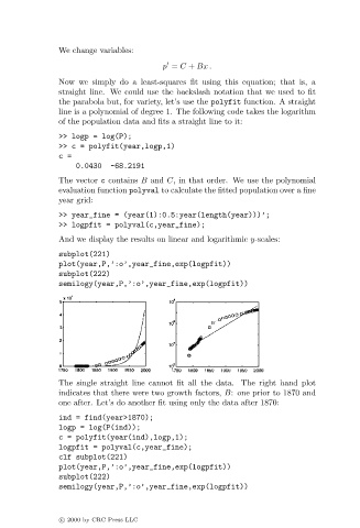
And we display the results on linear and logarithmic y-scales:

subplot(221)
plot(year,P,’:o’,year_fine,exp(logpfit))
subplot(222)
semilogy(year,P,’:o’,year_fine,exp(logpfit))

The single straight line cannot fit all the data. The right hand plot
indicates that there were two growth factors, B: one prior to 1870 and
one after. Let’s do another fit using only the data after 1870:
ind = find(year>1870);
logp = log(P(ind));
c = polyfit(year(ind),logp,1);
logpfit = polyval(c,year_fine);
clf subplot(221)
plot(year,P,’:o’,year_fine,exp(logpfit))
subplot(222)
semilogy(year,P,’:o’,year_fine,exp(logpfit))

c 2000 by CRC Press LLC