Page 197 - Basics of MATLAB and Beyond

If you zoom in on the right hand plot you’ll find that this growth rate is
too fast for the period between 1990 and 1996.

Exercise 5 (Page 55)

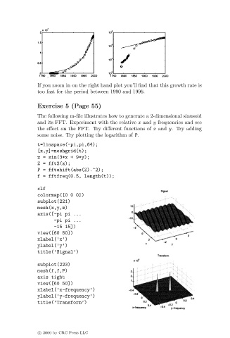
The following m-file illustrates how to generate a 2-dimensional sinusoid
and its FFT. Experiment with the relative x and y frequencies and see
the effect on the FFT. Try different functions of x and y. Try adding
some noise. Try plotting the logarithm of P.
t=linspace(-pi,pi,64);
[x,y]=meshgrid(t);
z = sin(3*x + 9*y);
Z = fft2(z);
P = fftshift(abs(Z).^2);
f = fftfreq(0.5, length(t));

clf
colormap([0 0 0])
subplot(221)
mesh(x,y,z)
axis([-pi pi ...
-pi pi ...
-15 15])
view([60 50])
xlabel(’x’)
ylabel(’y’)
title(’Signal’)

subplot(223)
mesh(f,f,P)
axis tight
view([60 50])
xlabel(’x-frequency’)
ylabel(’y-frequency’)
title(’Transform’)

c 2000 by CRC Press LLC