Page 163 - Biomedical Engineering and Design Handbook Volume 1, Fundamentals

140 BIOMECHANICS OF THE HUMAN BODY

that the front and back ends of the raw data were padded). This raises an interesting question, that
is, how do we identify an appropriate cutoff frequency for the filter? There are a number of methods
that can be used to help select an appropriate cutoff frequency. An FFT can be used to examine the
content of the signal in the frequency domain, or one of several residual analysis methods can be
used (Jackson, 1979; Winter, 1990).

6.4.2 Tracking Motion of the Segment and Underlying Bone
We continue with our example of how motion data collected with a video-based tracking system is
used in an inverse dynamics analysis. Calculating joint kinetics from the observed kinematics and
the external forces acting on the body requires knowledge of how the bones are moving. In this
section, we describe how tracking targets attached to the segments can be used to track motion of
the underlying bones. We assume the target coordinates have been smoothed using an appropriate
method.
The first step in calculating joint and segmental kinematics is to define orthogonal anatomical
coordinate systems (ACSs) embedded in each segment. Because it is the kinematics of the underlying
bones that are most often of interest, we must define a set of reference axes that are anatomically
meaningful for the purposes of describing the motion. An ACS is constructed for each segment in
the kinematic chain. Retroreflective targets positioned over anatomical sites (hence the term
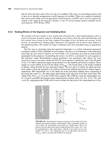
anatomical targets) are used to define the ACS for each segment. Consider the case in the left panel
of Fig. 6.10 where anatomical targets are positioned over the malleoli and femoral condyles. These
targets are used to define an ACS for the shank (ACS shank ). The frontal plane of the shank is defined
by fitting a plane through the four anatomical targets. The next step is to define the ankle and knee
joint centers, which are assumed to lie midway between the malleoli and femoral condyle targets,
respectively. The longitudinal axis of the shank lies in the previously defined plane, originating at
the distal joint center (i.e., the ankle joint) and pointing in the direction of the knee joint center. The
origin of the ACS shank is set at the COM of the segment. The COM lies along the longitudinal axis,
at a location generally determined using anthropometric lookup tables (see Sec. 6.4.4). The unit
vector X , originating at the COM will be used to define the direction of the longitudinal axis of the
s

X X

Z
Y Y

ACS shank

FIGURE 6.10 Retroreflective targets are placed over the medial and lateral
malleoli and femoral condyles (see left panel). These anatomical targets are
used to define the frontal plane of the shank (see middle panel). The X axis
projects from the ankle joint center towards the knee joint center. The Y axis
lies perpendicular to the frontal plane, with the Z axis given by the cross
product of X and Y. The orthogonal axes in the right panel represent the
ACS which is located at the COM of the segment.
shank