Page 158 - Biomedical Engineering and Design Handbook Volume 1, Fundamentals

BIOMECHANICS OF HUMAN MOVEMENT 135

In recent years, the so-called wand or dynamic calibration method has become widely used in place
of hanging strings with control points. In a dynamic calibration, two retroreflective targets attached to
a wand are moved throughout the entirety of the volume in which the movement will take place. The
targets on the wand are not control points per se because their locations in object-space are not known
a priori. However, since the coordinates of the two wand targets can be measured with respect to the
u, v coordinates of each camera and because the distance between targets should remain constant, the
cameras can be calibrated in an iterative manner until the length of the wand as detected by the cameras
matches the true length of the wand (i.e., distance between targets). Although the length of the wand
can be reconstructed very accurately using this method, the direction of the object-space reference axes
does not have to be known for determining the length. A static frame with a predefined origin and
control points arranged to define the object-space reference axes is placed in the field of view of the
“calibrated” cameras to establish the direction of the X, Y, Z object-space axes.

Calculating Object-Space Coordinates. Once
the cameras have been calibrated and a set of betas X, Y, Z
for each camera are known, the opposite approach
can be used to locate the position of a target in
object-space. The term reconstruction is often used Camera 2
to describe the process of calculating three- (u , v )
2
2
dimensional coordinates from multiple (n ≥ 2)
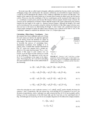
camera views. Consider the example illustrated in
Fig. 6.7, where two cameras have a unique per-
spective of the same tracking target. The u, v coor-
dinates of the target in each camera view are Camera 1
known, as are the betas for both cameras as a result (u , v )
1
1
of the calibration. The unknowns in this case are FIGURE 6.7 Cameras 1 and 2 each have a unique
the X, Y, Z coordinates of the target in the object- perspective of the tracking target in object-space (i.e.,
space. Rearranging Eq. (6.7) and (6.8) and adding silver circle). The X, Y, Z coordinates of the target can be
two more equations for the second camera leads to calculated using the u, v coordinates and the betas deter-
the following: mined during calibration.
1 32)
1 31)
'
'
u =(β ' 11 − u β ' X +(β 12 − u β ' Y + β ( 13 − u β '' ' 14 (6.9)
1 33) +Z β
1
1 31)
1 32)
1 33) +Z β
v =(β ' 21 − v β ' X +(β ' 22 − v β ' Y + β ( ' 23 − v β ' ' ' 24 (6.10)
1
2 32)
233)
2 31)
''
+
u =(β '' 11 − u β '' X +(β '' 12 − u β '' Y + β ( 13 − u β '' Z β '' 14 (6.11)
u
2
2 32)
233)
2 31)
''
+
v =(β 21 − v β '' X +(β '' 22 − v β '' Y + β ( '' 23 − v β '' Z β '' 24 (6.12)
v
2
where the subscript on u and v indicates camera 1 or 2, with β ' ij and β '' ij used to identify the betas for
cameras 1 and 2, respectively. We can express Eqs. (6.9) through (6.12) compactly if we let C ij be
the terms in parentheses, where i indicates row and j column [see Eq. (6.13) for an example], and by
letting L be the combination of the left-hand side and the lone beta on the right-hand side of
i
Eqs. (6.9) through (6.12) [see Eq. (6.14) for an example]. Equation (6.15) reflects this compact notation.
1 31)
'
C =(β 11 − u β ' (6.13)
11
L = ( u − ) (6.14)
''
β
14
2
3