Page 162 - Biomedical Engineering and Design Handbook Volume 1, Fundamentals

BIOMECHANICS OF HUMAN MOVEMENT 139

be in part why it is so widely used. Although we described the role of the Butterworth filter as
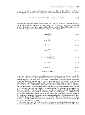
extracting particular frequencies, the raw signal is actually filtered in the time domain as seen below.

Yt() = a X t() + a X t −1 ) + a X t − 2 ) + b Yt −1 ) + b Y(t − 2) (6.19)
(
(
t
(
0
1
2
1
2
where Y(t) and X(t) are the filtered and raw data at time t. The (t × 1) and (t × 2) notation is used to
indicate data at 1 and 2 samples prior to the current time. Equation (6.19) is for a second-order
recursive filter; higher-order filters require additional recursive terms. The a and b coefficients for a
Butterworth low-pass filter can be determined using the following equations:
⎛ π f ⎞
c
ω = tan ⎜ ⎝ f s ⎠ ⎟ (6.20)
c
K = 2ω c (6.21)
1
K =ω 2 c (6.22)
2
2 a
K = 0 (6.23)
3
K 2
K
a = a = 2 (6.24)
0
2
( 1+ K + K )
2
1
a = 2 a 0 (6.25)
1
b =− 2 a + K 3 (6.26)
0
1
b =− a − K 3 (6.27)
12
2
0
where f and f are the cutoff frequency and the sampling frequency expressed in hertz, respectively.
c s
Several practical considerations should be noted when using a Butterworth digital filter. First, we
see from Eq. (6.19) that the filtered data at time t are related in a recursive manner to raw and
filtered data at times (t × 1) and (t × 2). This can cause problems at the beginning of the data set
unless the front end of the data is padded with extra data points. The bold line in Fig. (6.9) illustrates
the consequence of not padding the data set prior to filtering. Clearly the smoothed data at the beginning
(and also at the end!) of the data set are erroneous. Two methods of padding the front end of the data
involve reflecting the first n data points (15 or more generally work well for a second-order filter)
about data point #1, or simply by collecting more data than is actually needed. It should be noted
that this type of digital filter introduces a phase lag in the smoothed signal. The easiest method of
correcting for this phase lag is to refilter the already filtered data in the reverse direction. This will
shift the data in an equal and opposite direction, realigning the raw and filtered data temporally. Note
that filtering the already filtered data in the reverse direction will increase the sharpness of the filter
response. If the data are filtered in the reverse direction, it is advisable to pad the back end of the
data set for the reasons cited earlier.
The smooth thin line in Fig. 6.9 is the result of filtering the raw data in the forward and reverse
directions using a fourth-order, low-pass Butterworth filter set at a cutoff frequency of 6 Hz (note