Page 165 - Biomedical Engineering and Design Handbook Volume 1, Fundamentals

142 BIOMECHANICS OF THE HUMAN BODY

The relative position and orientation of the local coordinate system and the ACS can be repre-
sented as a translation vector relating their origins and a rotation matrix of direction cosines.
Moreover, the relative position and orientation between the local coordinate system and the ACS
should not change if we assume the segment is rigid. This relationship can be used to estimate the
position and orientation of the ACS at any point in time by tracking motion of targets attached to the
segment. This idea is easily expanded to multiple segments and forms the basis for comparing
relative motion between adjacent bones (i.e., ACSs).
Constructing a local coordinate system for the purposes of estimating motion of the ACS is a
straightforward and convenient method. However, the position and orientation of the local coordinate
system is generally sensitive to errors in the coordinates of the tracking targets, and therefore, the
estimated position and orientation of the ACS will also be affected. For this reason, it is generally
advantageous to use more than three targets per segment and a least squares method to track motion
of the segment and underlying bone. The singular value decomposition (SVD) method has been used
to this end with good success (Soderkvist & Wedin, 1993; Cheze et al., 1995). The SVD method
maps all of the tracking targets (n ≥ 3) from position a to position b using a least squares approxi-
mation. This is illustrated schematically in Fig. 6.13 and represented algebraically in Eq. (6.31).

[R] n 2
min ∑ Ra +− b i (6.31)
d
i
i=1
where n represents the number of targets attached to
d the segment, with a and b used to indicate the
i
i
object-space coordinates of the individual tracking
targets. R is a 3 × 3 rotation matrix, while d is a
Position b
Position a displacement vector that, when combined with R,
maps all targets in a least squares sense from their
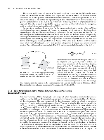
FIGURE 6.13 Least squares mapping of the tracking position in a to their position in b. Because the
targets from position a to position b. R is a 3 × 3 coordinates of the tracking targets are also known
rotation matrix and d is a displacement vector. relative to the ACS, the same least squares approach
can be used to determine how the ACS moved
between position a and position b. Note that although
this example maps the targets on the same segment, this idea can also be used to determine relative
kinematics between adjacent segments (cf. Soderkvist & Wedin, 1993).

6.4.3 Joint Kinematics: Relative Motion between Adjacent Anatomical
Coordinate Systems
It is clear from Fig. 6.11 that changing the knee angle will affect the relative orientation between the
ACS and the ACS . The orientation at any point in time can be represented by a 3 × 3 matrix
shank thigh
of direction cosines. The nine elements of the direction cosine matrix are related to an ordered
sequence of rotations about a particular set of axes. This can be visualized by starting out with the
ACS and ACS initially aligned, moving the ACS into its final orientation relative to the
shank thigh shank
ACS by rotating about the ZY X, ′ , ′′ axes of a moving reference frame. The ACS is the moving
thigh shank
reference in our example. The prime superscripts indicate that the orientation of the primed axes is
related to a previous rotation. The first rotation in the ZY X, ′ , ′′ sequence takes place about the ML
axis of the ACS thigh (or equivalently about the Z axis of the ACS shank because both ACSs are aligned at
the onset!). The Y′ axis about which the second rotation occurs is perpendicular to both the ML axis
of the thigh and the longitudinal axis of the shank. This mutually perpendicular axis is often called
the line of nodes (or floating axis in joint coordinate system terminology). The line of nodes is
formed by the vector cross product of the ML axis of the thigh and the longitudinal axis of the shank.
The final rotation takes place about the longitudinal axis of the shank (i.e., ′′ ). Note the double
X
superscript indicating the orientation of the longitudinal axis has been influenced by two previous
rotations about the Z and Y′ axes. These ordered rotations are known as Euler ZY X, ′ , ′′ angles. The