Page 203 - Biomedical Engineering and Design Handbook Volume 1, Fundamentals

180 BIOMECHANICS OF THE HUMAN BODY

subject to the equality constraints given by the dynamical equations of motion [Eqs. (7.7) and (7.1),
respectively]:

m
F MT = f F ( MT l , MT v , MT a , m ) 0 ≤ a ≤1
and

2
M()qq + C()qq + G () + R() F MT + E (, ) = 0
q
q
q
q
the initial states of the system,
,
MT
x() = x o x ={ q q F } (7.15)
0
,
and any terminal and/or path constraints that must be satisfied additionally. The dynamic optimiza-
tion problem formulated above is a two-point, boundary-value problem, which is often difficult to
solve, particularly when the dimension of the system is large (i.e., when the system has many dof
and many muscles).
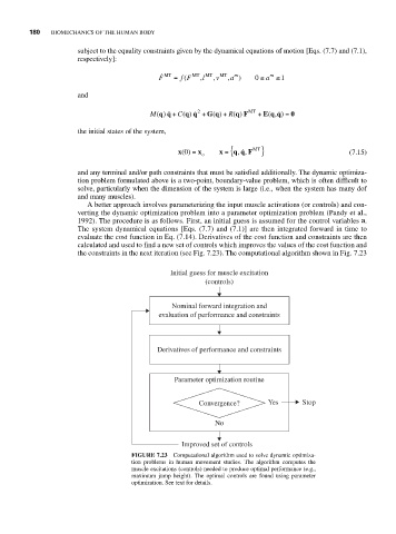
A better approach involves parameterizing the input muscle activations (or controls) and con-
verting the dynamic optimization problem into a parameter optimization problem (Pandy et al.,
1992). The procedure is as follows. First, an initial guess is assumed for the control variables . a
The system dynamical equations [Eqs. (7.7) and (7.1)] are then integrated forward in time to
evaluate the cost function in Eq. (7.14). Derivatives of the cost function and constraints are then
calculated and used to find a new set of controls which improves the values of the cost function and
the constraints in the next iteration (see Fig. 7.23). The computational algorithm shown in Fig. 7.23

Initial guess for muscle excitation
(controls)

Nominal forward integration and
evaluation of performance and constraints

Derivatives of performance and constraints

Parameter optimization routine

Convergence? Yes Stop

No

Improved set of controls
FIGURE 7.23 Computational algorithm used to solve dynamic optimiza-
tion problems in human movement studies. The algorithm computes the
muscle excitations (controls) needed to produce optimal performance (e.g.,
maximum jump height). The optimal controls are found using parameter
optimization. See text for details.