Page 322 - Biomedical Engineering and Design Handbook Volume 1, Fundamentals

ELECTROMYOGRAPHY AS A TOOL TO ESTIMATE MUSCLE FORCES 299

Forward dynamics Joint angle

Muscle a(t) Muscle F Musculoskeletal
EMG activation contraction geometry M F
dynamics dynamics (moment arms)

Output:
2
2
Alter model Σ (M F – M I ) ≠ 0 Moment Σ (M F – M I ) =0 muscle forces
parameters comparison optimized
parameters
Tuning process
Inverse dynamics
. ..
Position θ d θ d θ Equations
data dt dt of motion M I

Ground
F x , F y , F z , M x , M y , M z
reaction
force data

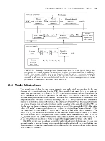
FIGURE 12.9 Theoretical flow of the hybrid forward-inverse dynamics model. Legend: EMG = elec-
tromyograms; a(t) = muscle activation; F = muscle force; M = joint moment calculated from forward dynam-
F
ics; M = joint moment calculated from inverse dynamics; θ (and derivatives) = joint angle, joint angular
I
velocity, joint angular acceleration; F ,F ,F ,M ,M ,M = ground reaction forces and moments in all three
x y z x y z
directions. In this model, M was used as a reference baseline, and we used a tuning process to optimize the
F
parameters of forward dynamics model such that M matches M .
F I
12.4.4 Model of Calibration Process
This model uses a hybrid forward-inverse dynamics approach, which assumes that the forward
dynamic joint moments estimated from the EMG-driven model should equal the joint moments esti-
mated from inverse dynamics, as shown in Fig. 12.9. A tuning process can then be used to calibrate the
model and obtain a set of model parameters for each subject to accurately estimate the knee joint
moments during five different calibration trials. Calibration tasks should be chosen to encompass a wide
range of contractile conditions. Simulated annealing (Goffe et al., 1994) is an often-used optimization
method to alter model parameters to minimize the difference between forward dynamic joint moments
and inverse dynamic joint moments. Simulated parallel annealing within a neighborhood (SPAN) can
also be used on clusters to improve the computational speed (Higginson et al., 2005). The initial
values of l s t and I for each muscle is necessary and can be obtained from Yamaguchi et al. (1990),
m
o
and constrained to change within ±15 percent and ±5 percent of their initial values, respectively. The
ranges of γ , γ , and A were described before, and the range of d should be approximately 10 to 100 ms
1 2
(Hull and Hawkins, 1990). Strength factors can be set to be within approximately 0.5 to 2.0, and the
F for each muscle can also be obtained from Yamaguchi et al. (1990). The initial values for γ , γ , d,
max 1 2
A, and strength factors can be set to be the average of their upper and lower limits (Table 12.1).
This EMG-driven knee model can account for different activation strategies and produce joint
moments similar to inverse dynamic joint moments during different tasks. It can be verified that once
the parameters are tuned, the model can then be used to predict joint moments of new tasks with new
muscle activation patterns.