Page 323 - Biomedical Engineering and Design Handbook Volume 1, Fundamentals

300 BIOMECHANICS OF THE HUMAN BODY

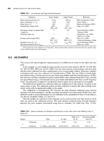
TABLE 12.1 Lower Bound and Upper Bound Parameters
Parameter Lower bound Upper bound Reference
Electromechanical delay (d) 10 ms 100 ms Hull and Hawkins (1990)
Filter coefficients (γ , γ ) −0.95 0.90 Cohen (2004)
1 2
Shape factor (A) 0.01 0.12 Manal and Buchaan (2003)
Optimal fiber length (OFL) OFL − OFL + Delp et al. (1990)
.
.
OFL 0.05 OFL 0.05
Percentage change in optimal fiber 0 0.25 Lloyd and Besier (2003),
length (λ) Huijing (1996)
Pennation angle (ϕ) * * Yamaguchi et al. (1990),
Delp et al. (1990)
Resting tendon length (RTL) RTL − RTL − Delp et al. (1990),
i
i
.
RTL . 0.15 RTL 0.15 Lloyd and Buchanan (1996)
i i
Strength factors (G , G ) F . 0.05 F . 0.02 Lloyd and Besier (2003)
f e max max
Maximum isometric force (F ) * * Delp et al. (1990)
max
All the parameters to be calibrated were listed above. Those labeled with an asterisk (*) have been fixed at a specific value,
which could be found in the listed literature.
12.5 AN EXAMPLE
This section will step through the implementation of an EMG-driven model for the ankle and knee
joint.
In this example, we will include the major muscles across the ankle and knee: RF, VL, VI, VM, MG,
LG, SM, ST, BFL, BFS, Sol, and TA. EMGs from the major muscles, joint positions, and force plate
data have been collected from three walking trials on two young healthy subjects. Maximum voluntary
contraction trials were also collected for normalization of EMG. The raw EMG are firstly high-
pass-filtered using a forward and reverse pass fourth-order Butterworth filter (cutoff frequency 50 Hz),
then full wave rectified, normalized by peak rectified EMG values obtained from MVC trials, and then
low-pass-filtered using a forward and reverse pass fourth-order Butterworth filter (cutoff frequency
6 Hz). The ankle joint of subject #1 and the knee joint of subject #2 are illustrated as an example.
The EMG-driven models are calibrated using one walking trial of the subjects, focusing on the
stance phase of gait. The calibrated models are then employed to predict the other walking trials,
which could verify the predictable ability of the model.
2
The coefficients of determination (R ) between the joint moments estimated using forward
dynamics and inverse dynamics, and the associated normalized root-mean-square (RMS) error (nor-
malized to peak-to-peak joint moment) for all calibration trials and prediction trials of both subjects,
can then be calculated (Tables 12.2 and 12.3).
Once the models are calibrated, joint moments can be predicted from new data based on novel
tasks not used in the calibration process. The joint moment predicted using forward dynamics
matched the joint moment determined using inverse dynamics for both trials (Fig. 12.10a,

TABLE 12.2 Statistical Results of Calibration and Prediction on the Ankle Joint of the Walking Trials of
Subject #1
RMS error Normalized RMS
.
2
Subject Trial R value (N m) error (%)
Calibration 1 0.935 9.61 6.30
1
Prediction 2~3 (Mean value (SD)) 0.939 (0.021) 8.98 (2.78) 6.20 (2.13)