Page 128 - Chemical Process Equipment - Selection and Design

100 FLOW OF FLUIDS

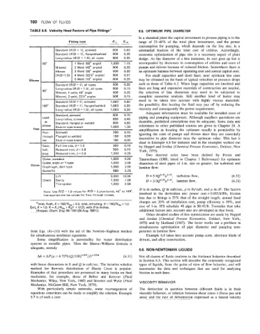
TABLE 6.6. Velocity Head Factors of Pipe Fittingsa 6.5. OPTIMUM PIPE DIAMETER
In a chemical plant the capital investment in process piping is in the
- --
range of 25-40% of the total plant investment, and the power
consumption for pumping, which depends on the line size, is a
Standard (RID = 11, screwed 800 0.40 substantial fraction of the total cost of utilities. Accordingly,
Standard (RID = 11, flangedIwelded 800 0.25 economic optimization of pipe size is a necessary aspect of plant
Long-radius (RID = 1.5), all types 800 0.20 design. As the diameter of a line increases, its cost goes up but is
90" 1 Weld (90" angle) 1,000 1.15 accompanied by decreases in consumption of utilities and costs of
Mitered 2 Weld (45" angles) 800 0.35 pumps and drivers because of reduced friction. Somewhere there is
elbows 3 Weld (30' angles) 800 0.30 an optimum balance between operating cost and annual capital cost.
(RID=1.5) 4 Weld (22%' angles) 800 0.27 For small capacities and short lines, near optimum line sizes
Elbow! 5 Weld (18" angles) 800 0.25 may be obtained on the basis of typical velocities or pressure drops
Standard (RID = l), all types 500 0.20 such as those of Table 6.2. When large capacities are involved and
Long-radius (RID = 1.51, all types 500 0.15 lines are long and expensive materials of construction are needed,
450 the selection of line diameters may need to be subjected to
Mitered, 1 weld, 45" angle 500 0.25
Mitered, 2 weld, 22%" angles 500 0.15 complete economic analysis. Still another kind of factor may
Standard (RID = 1 ), screwed 1,000 0.60 need to be taken into account with highly viscous materials:
the possibility that heating the fluid may pay off by reducing the
180"
- Standard (RID = 1 ), flanged/welded 1,000 0.35 viscosity and consequently the power requirement.
0.30
1,000
Long radius (RID = 1.51, all types
Standard, screwed 500 0.70 Adequate information must be available for installed costs of
Used Long-radius, screwed 800 0.40 piping and pumping equipment. Although suppliers quotations are
as Standard, flanged or welded 800 0.80 desirable, published correlations may be adequate. Some data and
'Ibow Stub-in-type branch 1,000 1.00 references to other published sources are given in Chapter 20. A
Tee! simplification in locating the optimum usually is permissible by
Run- Screwed 200 0.10 ignoring the costs of pumps and drivers since they are essentially
150
through Flanged or welded
- Stub-in-type branch 100 0.50 insensitive to pipe diameter near the optimum value. This fact is
0.00
tee
clear in Example 6.8 for instance and in the examples worked out
Gate, Full line size, 0 = 1 .O 300 0.10 by Happel and Jordan (Chemical Process Economics, Dekker, New
ball, Reduced trim, p = 0.9 500 0.15 York, 1975).
plug Reduced trim, p = 0.8 1,000 0.25 Two shortcut rules have been derived by Peters and
Timmerhaus (1980; listed in Chapter 1 References) for optimum
diameters of steel pipes of 1-in. size or greater, for turbulent and
Valve
laminar flow:
Lift 2,000 10.00 D = 3.9Q0.45p0.'3, turbulent flow, (6.32)
,
Check Swing 1,500 1.50 D = 3.0~0.36~0.18 laminar flow. (6.33)
Tilting-disk 1,000 0.50
D is in inches, Q in cuft/sec, p in lb/cuft, and p in cP. The factors
involved in the derivation are: power cost = 0.055/kWh, friction
loss due to fittings is 35% that of the straight length, annual fixed
charges are 20% of installation cost, pump efficiency is 50%, and
ahlet, flush, K = 160/N,, + 0.5. Inlet, intruding, K = 160/NR,= 1.0.
Exit, K= 1.0. K = K,/NRe + K,(1 + l/D), with Din inches. cost of 1-in. IPS schedule 40 pipe is $0.45/ft. Formulas that take
[Hooper, Chern. Eng. 96-100 (24Aug. 1981)l. additional factors into account also are developed in that book.
Other detailed studies of line optimization are made by Happel
and Jordan (Chemical Process Economics, Dekker, New York,
1975) and by Skelland (1967). The latter works out a problem in
simultaneous optimization of pipe diameter and pumping tem-
from Eqs. (4)-(10) with the aid of the Newton-Raphson method perature in laminar flow.
for simultaneous nonlinear equations. Example 6.8 takes into account pump costs, alternate kinds of
Some simplification is permissible for water distribution drivers, and alloy construction.
systems in metallic pipes. Then the Hazen-Williams formula is
adequate, namely
6.6. NON-NEWTONIAN LIQUIDS
Ah = AP/p = 4.727L(Q/130)1~852/D4.8704 (6.31) Not all classes of fluids conform to the frictional behavior described
in Section 6.3. This section will describe the commonly recognized
with linear dimensions in ft and Q in cuft/sec. The iterative solution types of liquids, from the point of view of flow behavior, and will
method for flowrate distribution of Hardy Cross is popular. summarize the data and techniques that are used for analyzing
Examples of that procedure are presented in many books on fluid friction in such lines.
mechanics, for example, those of Bober and Kenyon (Fluid
Mechanics, Wiley, New York, 1980) and Streeter and Wylie (Fluid VISCOSITY BEHAVIOR
Mechanics, McGraw-Hill, New York, 1979).
With particularly simple networks, some rearrangement of The distinction in question between different fluids is in their
equations sometimes can be made to simplify the solution. Example viscosity behavior, or relation between shear stress z (force per unit
6.7 is of such a case. area) and the rate of deformation expressed as a lateral velocity