Page 291 - Computational Retinal Image Analysis

4 Clinical applications 289

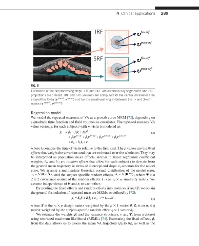
FIG. 8
Illustration of the preprocessing steps. IRF and SRF are automatically segmented and 2D
projections are created. IRF and SRF volumes are computed for the central millimeter area
around the fovea (v fov-irf , v fov-srf ) and for the parafoveal ring in-between the 1- and 3-mm
radius (v para-irf , v para-srf ).

Regression model
We model the repeated measures of VA as a growth curve MRM [72], depending on
a quadratic time function and fluid volumes as covariates. The repeated-measure VA
value vector, y, for each subject i with n i visits is modeled as:
y i = β 0 + β 1 t + β 2 t 2 i (2)
i
+ β v fovirf + β v fov srf + β v parairf + β v para--srf
-
-
-
3 4 5 6
+ b + b t i i + ε , i
i 0
1
where t i contains the time of visits relative to the first visit. The β values are the fixed
effects that weight the covariates and that are estimated over the whole set. They may
be interpreted as population mean effects, similar to linear regression coefficient
weights. b 0i and b 1i are random effects that allow for each subject i to deviate from
the general mean trajectory in terms of intercept and slope. ε i accounts for the model
error. We assume a multivariate Gaussian normal distribution of the model error,
0
2
ε ∼  (, σ I ) , and the subject-specific random effects, b ∼  (,Ψ ) , where Ψ is a
0
i i
2 × 2 covariance matrix of the random effects. I is an n i × n i similarity matrix. We
assume independence of b i and ε i to each other.
By pooling the fixed effects and random effects into matrices X and Z, we obtain
the general formulation of repeated measure MRMs as defined by [72]:
y = X β + Z b + ε , i = …,,
1
N
,
i i ii i (3)
where X is the n i × p design matrix weighted by the p × 1 vector β. Z i is an n i × q
matrix weighted by the subject-specific random effect q × 1 vector b i .
We estimate the weights, β, and the variance structures, σ and Ψ, from a dataset
using restricted maximum likelihood (REML) [74]. Estimating the fixed effects, β,
from the data allows us to assess the mean VA trajectory (β 0 to β 2 ), as well as the