Page 290 - Computational Retinal Image Analysis

288 CHAPTER 14 OCT fluid detection and quantification

100 IRF 0 m m ³ 1 m m ³
Visual acuity (letters) 60 SRF
80

90
40
50
20 VA 70
0 100 200 300 0 60 120 180 240 300 360
(A) Days (B) Days
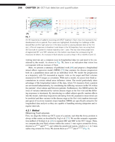
FIG. 7
(A) VA trajectories of patients receiving anti-VEGF treatment. Each blue line represents the
development of one patient. Four cases are highlighted, illustrating the challenge in this
dataset that are the high variance in the data caused by varying disease state at the first
visit, different responses to treatment and drops in the VA trajectory from recurring fluid.
(B) Example of a patient’s disease trajectory over 1 year. The top rows show projections
of segmented IRF and SRF volumes and the bottom row shows the corresponding VA
measured in letters. An increase in fluid volume caused a drop in VA at months 6 and 10.

visiting intervals are a common issue in longitudinal data too and need to be con-
sidered by the model. As shown in Fig. 7B, there is an indication that vision loss
corresponds with an increase of fluid.
Here, we present a summary of published work [68] and propose a longitudinal
mixed effects regression model (MRM) [72] that captures the disease progression
both on a population mean and on an individual level. We model the progression
as a trajectory with VA measured at regular visits as the target and fluid volumes
measured in OCT images as covariates. With such a model, we assess how fluid ac-
cumulations in certain retinal areas influence vision. The model particularly takes
advantage of the longitudinal nature of the data, where VA measures from a patient
are not treated independently, by considering the differing variances in the VA within
the patients’ observations and between patients. Furthermore, this MRM tackles the
issue of variance introduced by various disease stages at the first visit and the differ-
ing responses to treatment. By introducing so-called subject-specific random effects
into the model, individual trajectories deviating from the population mean trend can
be modeled and thus variance in the disease stage at the first visit (random intercept)
and speed of recovery (random slope) handled. MRMs are specifically attractive for
longitudinal data analysis as they are capable of handling missing datapoints and ir-
regular intervals.

4.2.1 Method
Obtaining fluid volumes
First, we align the follow-up OCT scans of a patient, such that the fovea position is
always at the center, as described by Vogl et al. [73]. We use the semantic segmenta-
tion method of Schlegl et al. [21] to segment IRF and SRF in the OCT image. Then,
we compute the total fluid volume within the central 1-mm region around the fovea,
denoted as v fov-irf and v fov-srf , and within the parafoveal region, which is a 1- to 3-mm
radius ring around the fovea. We denote them as v para-irf and v para-srf (Fig. 8).