Page 129 - Computational Statistics Handbook with MATLAB

116 Computational Statistics Handbook with MATLAB

% Plot as density histogram - Equation 5.1.
bar(x,nu/(140*h),1)
hold on
plot(xp,yp)
xlabel(‘Length (inches)’)
title('Density Histogram and Density Estimate')
hold off
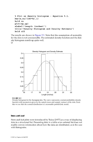
The results are shown in Figure 5.3. Note that the assumption of normality
for the data is not unreasonable. The estimated density function and the den-
sity histogram match up quite well.

Density Histogram and Density Estimate
0.4

0.35
0.3

0.25

0.2

0.15
0.1

0.05

0
16 17 18 19 20 21 22
Length (inches)

FI F U URE G 5. RE 5. 3 3
IG
F F II GU RE RE 5. 5. 3
3
GU
Density histogram for the forearm data. The curve represents a normal probability density
function with parameters given by the sample mean and sample variance of the data. From
this we see that the normal distribution is a reasonable probabilistic model.

Stem - -aandnd -LLeeaaf f
SStemtem
Stem
-
-- LLeeaaff
-- aandnd
Stem-and-leaf plots were introduced by Tukey [1977] as a way of displaying
data in a structured list. Presenting data in a table or an ordered list does not
readily convey information about how the data are distributed, as is the case
with histograms.

© 2002 by Chapman & Hall/CRC