Page 134 - Computational Statistics Handbook with MATLAB

Chapter 5: Exploratory Data Analysis 121

3

2

Y − Standard Normal −1
1

0

−2

−3
−3 −2 −1 0 1 2 3
X − Standard Normal
F FI U URE G 5. RE 5. 6 6
IG
6
GU
F F II GU RE RE 5. 5. 6
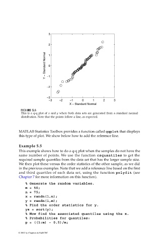
This is a q-q plot of x and y where both data sets are generated from a standard normal
distribution. Note that the points follow a line, as expected.
MATLAB Statistics Toolbox provides a function called qqplot that displays
this type of plot. We show below how to add the reference line.

Example 5.5
This example shows how to do a q-q plot when the samples do not have the
same number of points. We use the function csquantiles to get the
required sample quantiles from the data set that has the larger sample size.
We then plot these versus the order statistics of the other sample, as we did
in the previous examples. Note that we add a reference line based on the first
and third quartiles of each data set, using the function polyfit (see
Chapter 7 for more information on this function).
% Generate the random variables.
m = 50;
n = 75;
x = randn(1,n);
y = randn(1,m);
% Find the order statistics for y.
ys = sort(y);
% Now find the associated quantiles using the x.
% Probabilities for quantiles:
p = ((1:m) - 0.5)/m;

© 2002 by Chapman & Hall/CRC