Page 133 - Computational Statistics Handbook with MATLAB

120 Computational Statistics Handbook with MATLAB

We look first at the case where the sizes of the data sets are equal, so
m = n . In this case, we plot as points the sample quantiles of one data set
versus the other data set. This is illustrated in Example 5.4. If the data sets
come from the same distribution, then we would expect the points to approx-
imately follow a straight line.
A major strength of the quantile-based plots is that they do not require the
two samples (or the sample and theoretical distribution) to have the same
location and scale parameter. If the distributions are the same, but differ in
location or scale, then we would still expect the quantile-based plot to pro-
duce a straight line.

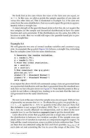
Example 5.4
We will generate two sets of normal random variables and construct a q-q
plot. As expected, the q-q plot (Figure 5.6) follows a straight line, indicating
that the samples come from the same distribution.

% Generate the random variables.
x = randn(1,75);
y = randn(1,75);
% Find the order statistics.
xs = sort(x);
ys = sort(y);
% Now construct the q-q plot.
plot(xs,ys,'o')
xlabel('X - Standard Normal')
ylabel('Y - Standard Normal')
axis equal
If we repeat the above MATLAB commands using a data set generated from
an exponential distribution and one that is generated from the standard nor-
mal, then we have the plot shown in Figure 5.7. Note that the points in this q-
q plot do not follow a straight line, leading us to conclude that the data are
not generated from the same distribution.

We now look at the case where the sample sizes are not equal. Without loss
of generality, we assume that m < n . To obtain the q-q plot, we graph the y i() ,
⁄
,
,
i = 1 … m against the i –( 0.5) m quantile of the other data set. Note that
⁄
this definition is not unique [Cleveland, 1993]. The i –( 0.5) m quantiles of
the x data are usually obtained via interpolation, and we show in the next
example how to use the function csquantiles to get the desired plot.
Users should be aware that q-q plots provide a rough idea of how similar
the distribution is between two random samples. If the sample sizes are
small, then a lot of variation is expected, so comparisons might be suspect. To
help aid the visual comparison, some q-q plots include a reference line. These
,
(
are lines that are estimated using the first and third quartiles q 0.25 q 0.75 ) of
each data set and extending the line to cover the range of the data. The

© 2002 by Chapman & Hall/CRC