Page 135 - Computational Statistics Handbook with MATLAB

122 Computational Statistics Handbook with MATLAB

3

2
Y − Standard Normal −1
1

0

−2

−3

−0.5 0 0.5 1 1.5 2 2.5 3 3.5 4 4.5 5
X − Exponential

U
F FI IG URE G 5. RE 5. 7 7
7
F F II GU RE RE 5. 5. 7
GU
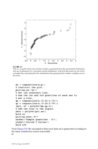
This is a q-q plot where one random sample is generated from the exponential distribution
and one is generated by a standard normal distribution. Note that the points do not follow
a straight line, indicating that the distributions that generated the random variables are not
the same.
xs = csquantiles(x,p);
% Construct the plot.
plot(xs,ys,'ko')
% Get the reference line.
% Use the 1st and 3rd quartiles of each set to
% get a line.
qy = csquantiles(y,[0.25,0.75]);
qx = csquantiles(x,[0.25,0.75]);
[pol, s] = polyfit(qx,qy,1);
% Add the line to the figure.
yhat = polyval(pol,xs);
hold on
plot(xs,yhat,'k')
xlabel('Sample Quantiles - X'),
ylabel('Sorted Y Values')
hold off
From Figure 5.8, the assumption that each data set is generated according to
the same distribution seems reasonable.

© 2002 by Chapman & Hall/CRC