Page 137 - Computational Statistics Handbook with MATLAB

124 Computational Statistics Handbook with MATLAB

tions, one can use the MATLAB code given below, substituting the appropri-
ate function to get the theoretical quantiles.

Example 5.6
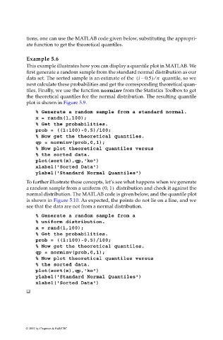
This example illustrates how you can display a quantile plot in MATLAB. We
first generate a random sample from the standard normal distribution as our
data set. The sorted sample is an estimate of the i –( 0.5) n quantile, so we
⁄
next calculate these probabilities and get the corresponding theoretical quan-
tiles. Finally, we use the function norminv from the Statistics Toolbox to get
the theoretical quantiles for the normal distribution. The resulting quantile
plot is shown in Figure 5.9.

% Generate a random sample from a standard normal.
x = randn(1,100);
% Get the probabilities.
prob = ((1:100)-0.5)/100;
% Now get the theoretical quantiles.
qp = norminv(prob,0,1);
% Now plot theoretical quantiles versus
% the sorted data.
plot(sort(x),qp,'ko')
xlabel('Sorted Data')
ylabel('Standard Normal Quantiles')
To further illustrate these concepts, let’s see what happens when we generate
a random sample from a uniform 01,( ) distribution and check it against the
normal distribution. The MATLAB code is given below, and the quantile plot
is shown in Figure 5.10. As expected, the points do not lie on a line, and we
see that the data are not from a normal distribution.
% Generate a random sample from a
% uniform distribution.
x = rand(1,100);
% Get the probabilities.
prob = ((1:100)-0.5)/100;
% Now get the theoretical quantiles.
qp = norminv(prob,0,1);
% Now plot theoretical quantiles versus
% the sorted data.
plot(sort(x),qp,'ko')
ylabel('Standard Normal Quantiles')
xlabel('Sorted Data')

© 2002 by Chapman & Hall/CRC