Page 141 - Computational Statistics Handbook with MATLAB
P. 141

128                        Computational Statistics Handbook with MATLAB


                                end
                                % Add some whitespace to see better.
                                axis([-0.5 max(k)+1 min(phik)-1 max(phik)+1])
                                xlabel('Number of Occurrences - k')
                                ylabel('\phi (n_k)')
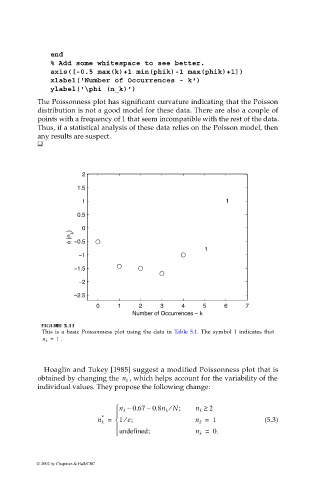
                             The Poissonness plot has significant curvature indicating that the Poisson
                             distribution is not a good model for these data. There are also a couple of
                             points with a frequency of 1 that seem incompatible with the rest of the data.
                             Thus, if a statistical analysis of these data relies on the Poisson model, then
                             any results are suspect.


                                         2
                                        1.5
                                         1                                       1

                                        0.5
                                         0
                                      φ (n k )  −0.5

                                                                           1
                                        −1
                                       −1.5
                                        −2

                                       −2.5
                                             0     1     2     3     4     5     6     7
                                                       Number of Occurrences − k

                               IG
                              FI F U URE G 5.  RE 5. 1  11 1
                              F F II  GU  RE RE 5. 5.  1 1 1
                               GU
                                     1
                              This is a basic Poissonness plot using the data in Table 5.1. The symbol  1 indicates that
                              n k =  1  .
                              Hoaglin and Tukey [1985] suggest a modified Poissonness plot that is
                                                      , which helps account for the variability of the
                             obtained by changing the  n k
                             individual values. They propose the following change:

                                                                  ⁄
                                                   n k –  0.67 –  0.8n k N;  n k ≥  2
                                                     ⁄
                                               *  
                                             n k =   1 e;               n k =  1           (5.3)
                                                  
                                                   undefined;           n =  0.
                                                                          k

                            © 2002 by Chapman & Hall/CRC
   136   137   138   139   140   141   142   143   144   145   146