Page 143 - Computational Statistics Handbook with MATLAB

130 Computational Statistics Handbook with MATLAB

1

0.5

0 1

−0.5
φ (n * ) k −1

−1.5
1
−2

−2.5
0 1 2 3 4 5 6 7
Number of Occurrences − k

F FI U URE G 5.1 RE 5.1 2 2
IG
5.1
GU
F F II GU RE RE 5.1 2 2
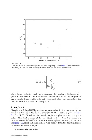
This is a modified Poissonness plot for the word frequency data in Table 5.1. Here the counts
where n k = 1 do not seem radically different from the rest of the observations.
 
 * 
n k
*
(

ϕ n k ) = ln  -------------------  ,  (5.4)
n 
 
 N ×  
  
k
*
along the vertical axis. Recall that n represents the number of trials, and n k is
given by Equation 5.3. As with the Poissonness plot, we are looking for an
*
(
approximate linear relationship between k and ϕ n k ) . An example of the
binomialness plot is given in Example 5.9.
Example 5.9
Hoaglin and Tukey [1985] provide a frequency distribution representing the
number of females in 100 queues of length 10. These data are given in Table
5.2. The MATLAB code to display a binomialness plot for n = 10 is given
below. Note that we cannot display ϕ n k ) for k = 10 (in this example),
*
(
because it is not defined for n k = 0 . The resulting binomialness plot is shown
in Figure 5.13, and it indicates a linear relationship. Thus, the binomial model
for these data seems adequate.
% Binomialness plot.

© 2002 by Chapman & Hall/CRC