Page 148 - Computational Statistics Handbook with MATLAB

Chapter 5: Exploratory Data Analysis 135

6
5

4
3
2
Values 1

0
−1
−2

−3

1 2 3
Column Number

U
FI F IG URE G 5.1 RE 5.1 5 5
F F II GU RE RE 5.1 5 5
5.1
GU
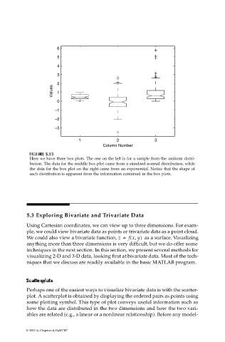
Here we have three box plots. The one on the left is for a sample from the uniform distri-
bution. The data for the middle box plot came from a standard normal distribution, while
the data for the box plot on the right came from an exponential. Notice that the shape of
each distribution is apparent from the information contained in the box plots.

5.3 Exploring Bivariate and Trivariate Data
Using Cartesian coordinates, we can view up to three dimensions. For exam-
ple, we could view bivariate data as points or trivariate data as a point cloud.
,
(
We could also view a bivariate function, z = f x y) as a surface. Visualizing
anything more than three dimensions is very difficult, but we do offer some
techniques in the next section. In this section, we present several methods for
visualizing 2-D and 3-D data, looking first at bivariate data. Most of the tech-
niques that we discuss are readily available in the basic MATLAB program.

Scaat
Sc
SSccaatt tterplotterplots terplotterplot ss s
Perhaps one of the easiest ways to visualize bivariate data is with the scatter-
plot. A scatterplot is obtained by displaying the ordered pairs as points using
some plotting symbol. This type of plot conveys useful information such as
how the data are distributed in the two dimensions and how the two vari-
ables are related (e.g., a linear or a nonlinear relationship). Before any model-

© 2002 by Chapman & Hall/CRC