Page 149 - Computational Statistics Handbook with MATLAB

136 Computational Statistics Handbook with MATLAB

ing, such as regression, is done using bivariate data, the analyst should
always look at a scatterplot to see what type of relationship is reasonable. We
will explore this further in Chapters 7 and 10.
A scatterplot can be obtained easily in MATLAB using the plot command.
One simply enters the marker style or plotting symbol as one of the argu-
ments. See the help on plot for more information on what characters are
available. By entering a marker (or line) style, you tell MATLAB that you do
not want to connect the points with a straight line, which is the default. We
have already seen many examples of how to use the plot function in this
way when we constructed the quantile and q-q plots.
An alternative function for scatterplots that is available with MATLAB is
the function called scatter. This function takes the input vectors x and y
and plots them as symbols. There are optional arguments that will plot the
markers as different colors and sizes. These alternatives are explored in
Example 5.11.

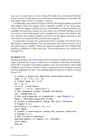
Example 5.11
We first generate a set of bivariate normal random variables using the tech-
nique described in Chapter 4. However, it should be noted that we find the
matrix R in Equation 4.19 using singular value decomposition rather than
Cholesky factorization. We then create a scatterplot using the plot function
and the scatter function. The resulting plots are shown in Figure 5.16 and
Figure 5.17.

% Create a positive definite covariance matrix.
vmat = [2, 1.5; 1.5, 9];
% Create mean at (2,3).
mu = [2 3];
[u,s,v] = svd(vmat);
vsqrt = ( v*(u'.*sqrt(s)))';
% Get standard normal random variables.
td = randn(250,2);
% Use x=z*sigma+mu to transform - see Chapter 4.
data = td*vsqrt+ones(250,1)*mu;
% Create a scatterplot using the plot function.
% Figure 5.16.
plot(data(:,1),data(:,2),'x')
axis equal
% Create a scatterplot using the scatter fumction.
% Figure 5.17.
% Use filled-in markers.
scatter(data(:,1),data(:,2),'filled')
axis equal
box on

© 2002 by Chapman & Hall/CRC