Page 147 - Computational Statistics Handbook with MATLAB

134 Computational Statistics Handbook with MATLAB

Possible Outliers
3

2

1

Values 0 Quartiles Adjacent
Values

−1

−2

−3

1
Column Number

U
FI F IG URE G 5.1 RE 5.1 4 4
5.1
GU
F F II GU RE RE 5.1 4 4
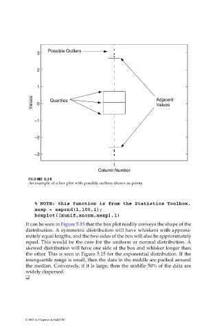
An example of a box plot with possible outliers shown as points.
% NOTE: this function is from the Statistics Toolbox.
xexp = exprnd(1,100,1);
boxplot([xunif,xnorm,xexp],1)
It can be seen in Figure 5.15 that the box plot readily conveys the shape of the
distribution. A symmetric distribution will have whiskers with approxi-
mately equal lengths, and the two sides of the box will also be approximately
equal. This would be the case for the uniform or normal distribution. A
skewed distribution will have one side of the box and whisker longer than
the other. This is seen in Figure 5.15 for the exponential distribution. If the
interquartile range is small, then the data in the middle are packed around
the median. Conversely, if it is large, then the middle 50% of the data are
widely dispersed.

© 2002 by Chapman & Hall/CRC