Page 152 - Computational Statistics Handbook with MATLAB

Chapter 5: Exploratory Data Analysis 139

0.14
0.12
0.1
0.08
0.06
0.04
0.02

2 3
2
0 1
0
−2 −2 −1
−3
IG
FI F U URE G 5.1 RE 5.1 8 8
5.1
GU
F F II GU RE RE 5.1 8 8
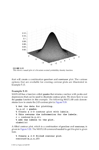
This shows a surf plot of a bivariate normal probability density function.
that will create a combination pcolor and contour plot. The various
options that are available for creating contour plots are illustrated in
Example 5.13.

Example 5.13
MATLAB has a function called peaks that returns a surface with peaks and
depressions that can be used to illustrate contour plots. We show how to use
the peaks function in this example. The following MATLAB code demon-
strates how to create the 2-D contour plot in Figure 5.19.

% Get the data for plotting.
[x,y,z] = peaks;
% Create a 2-D contour plot with labels.
% This returns the information for the labels.
c = contour(x,y,z);
% Add the labels to the plot.
clabel(c)
A filled contour plot, which is a combination of pcolor and contour, is
given in Figure 5.20. The MATLAB command needed to get this plot is given
here.
% Create a 2-D filled contour plot.
contourf(x,y,z,15)

© 2002 by Chapman & Hall/CRC